This wikilog article is a draft, it was not published yet.

Crash course in Scientific Computing

Revision as of 16:12, 8 March 2021

Crash Course in Scientific Computing

or, as officially known, The Wolverhampton Lectures on Physics: VI — Scientific Computing.

or do you mean

Crash course in Julia (programming)

When plotting pure functions, you might find that the density of points (PlotPoints in Mathematica) is not enough. This can be increased by specifying the step in the range, but in this case beware not to query your functions outside of its validity range, which would work otherwise. Compare:

plot(x->sqrt((15/x^2)-1),0,4,linewidth=5,linealpha=.5,linecolor=:red,ylims=(0,3))
plot!(x->sqrt((15/x^2)-1),0:.0001:3.8729,linewidth=2,linecolor=:blue,ylims=(0,3))

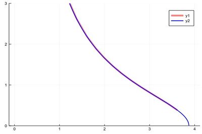
The first version can plot over the range 0–4 but does so by not plotting the full function, while the second (with x-steps of 0.0001 allowing for the nice curvature) shows everything but would return an error if going over the limit where the argument gets negative.

So much for integration.

Let us now turn to another typical numerical method: a root-finding algorithm. We used a so-called bisection method previously when generating our own random numbers, which is easy to implement but not very efficient. A simple but good improvement is the Newton–Raphson method (Newton used it for the particular case of polynomials; Raphson extended it to arbitrary functions). The idea is to start with a blind guess $x_0$ around the solution and replace the real function $f(x)$ by a linear approximation with the same slope at $x_0$, i.e., $h(x)=f'(x_0)x+\beta$ with $\beta$ such that $h(x_0)=f(x_0)$ which yields

$$h(x)=f'(x_0)[x-x_0]+f(x_0)$$

Now a better guess for the zero is found by solving $h(x)=0$ which has solution $x=x_0-(f(x_0)/f'(x_0))$. Of course the procedure can be iterated so the algorithm gives us the always better approximations:

$$x_{n+1}=x_n-{f(x_n)\over f'(x_n)}\,.$$

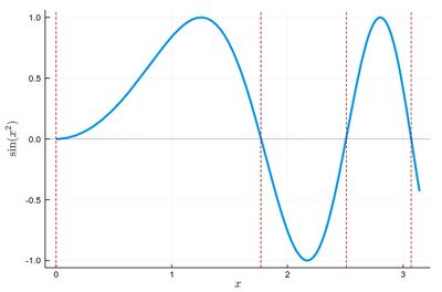
Let us find the zeros of $f(x)=\sin(x^2)$ between 0 and $\pi$. It's good to know beforehand the sort of results we expect (we added vertical lines by eye):

psin2=plot(x->sin(x^2), 0, π,
ylabel=L"\sin(x^2)",xlabel=L"x",lw=3,
legend=false)
vline!([0, 1.77, 2.51, 3.07], line = (:red, :dash, 1))
hline!([0], line = (:black, :dot, .75))

The formula gives us:

$$x_{n+1}=x_n-{\sin x_n^2\over 2x_n\cos x_n^2}$$

We can write a function that takes $f/f'$ as an input (that we have to compute ourselves) that computes such iterations until the procedure differs by less than some $\epsilon$:

function NewtonRaphson(f, x0)
    ϵ=10^-16
    x1=x0+10ϵ
    while abs(x1-x0)>ϵ
        x0=x1
        x1=x0-f(x0)
    end
    x1
end

This provides the values found in the $[0,\pi]$ interval:

lsols=[NewtonRaphson(x->sin(x^2)/(2*x*cos(x^2)), x) for x in 0:.01:π]

We can plot the solutions together with where was the starting point:

psin2=plot(x->sin(x^2), 0, π,
label=L"\sin(x^2)",xlabel=L"x",
legend=:bottomleft)

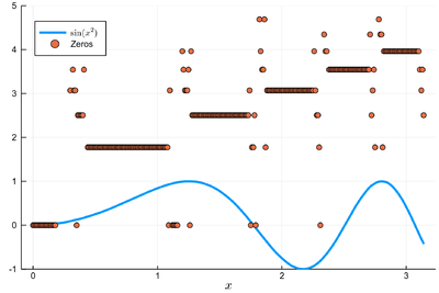
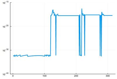
We found many, in particular some outside the $[0,\pi]$ range (this was the case when the tangent was sending us far away). We can check these are indeed all solutions:

plot(abs.(sin.(lsols.^2)), yscale=:log10, ylims=(10^-40,10^-10), legend=false)

To actually extract the values, we could use unique(), but this would return a lot of different values for the 0 zero, so we'd round this:

lsolss=sort(unique(round.(lsols,digits=10)))

These are the said solution in the sought range:

lsolss[findall(x-> 0<=x<=π, lsolss)]

5-element Array{Float64,1}:
 -0.0         
  0.0         
  1.7724538509
  2.5066282746
  3.0699801238

-0.0 and 0.0 are seen as different in julia, surely something that'll be fixed eventually. We have four solutions, as is clear from the initial graph.

There is a Roots package that has a function fzero() that achieves something similar:

fzero(x->sin(x^2), 2)

1.772453850905516

Let us now turn to a typical numerical problem, solving differential equations. We'll start with Ordinary Differential Equations (ODE). Namely, we consider equations of the type:

$$\tag{1} y'(t)=f(t,y(t))$$

The most famous algorithm is Euler's method and the most popular the RK4 variant of the Runge–Kutta methods. In between are a variety of possible implementations, many related in some way or the other. Methods can be explicit (the solution only depends on quantities already known) or implicit (the solution involves other unknowns which requires solving intermediate equations). The backward Euler method is an implicit method. Euler's method is the simplest one and the typical starting point to introduce the basic idea. Not surprisingly, it is also one of the least efficient. We discretize time into steps $t_1$, $t_2$, $\cdots$, $t_n$ separated by the same interval $h$. The solutions at these times are denoted $y_n=y(t_n)$. Back to (1), approximating $y'(t)\approx (y(t+h)-y(t))/h$, we have:

$$y_{n+1}=y_n+hf(t_n,y_n)$$

This is very simple since from the solution $y_n$ at time $t_n$ we can compute the solution at $t_{n+1}$. Explicitly.

Let us solve, for instance, $y'=-y$, whose solution is the exponential function.

npts = 100; # number of points
y=0.0*collect(1:npts); # predefine the array
h=.1; # timesteps, so total time = npts*h=10
# The differential equation to solve
function f(t,y)
    -y
end
y[1]=1; # initial condition
# The numerical method (Euler's)
for i=1:npts-1
    y[i+1]=y[i]+h*f((i-1)*h,y[i])
end

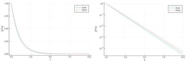
And we can now compare the numerical solution to the real one:

plot(((1:npts).-1)*h, [y[i] for i=1:npts], label="Euler", xlabel="t", ylabel="y'=-y")
plot!(x->exp(-x),0, 10, label="Exact")

Let us try the more difficult example:

$$y'={y\over 2}+2\sin(3t)\tag{2}$$

whose solution can be found with an integrating factor [1]

$$y=-{24\over37}\cos(3t)-{4\over37}\sin(3t)+\left(y(0)+{24\over 37}\right)e^{t/2}$$

In this case the differential equation is defined as:

function f(t,y)
    (y/2)+2sin(3t)
end

And the method can be quickly implemented as:

tmax=4*pi;
h=0.0001;
npts=round(Int64,tmax/h);
y=0.0*collect(1:npts);
y[1]=-24/37
for i=1:npts-1
    ti=(i-1)*h
    y[i+1]=y[i]+h*f(ti,y[i])
end

with various repetitions of

plot!(((1:npts).-1).*h, y,
    xlabel="t", ylabel="y", label="h=$(h)",
    legend=:bottomleft,ylims=(-2,.75),lw=3)

to see the effect of different time steps:

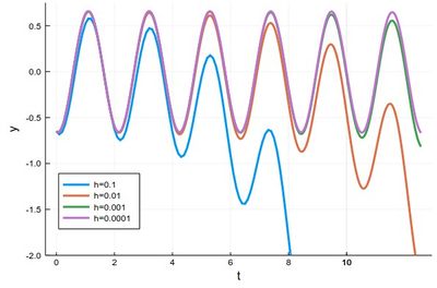
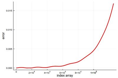
Comparing to the exact solution shows that the error gets quickly sizable, even with a lot of points:

plot(abs.([-(24/37)*cos(3t)-(4/37)*sin(3t) for t in ((1:npts).-1).*h]-y),
    lw=3, color=:red, xlabel="index array", ylabel="error", legend=false)

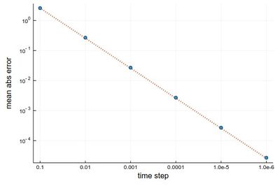
We can analyze the error in more details:

hlist=[10.0^(-k) for k=1:6];
herror=[];
for h in hlist
    npts=round(Int64,tmax/h);
    y=0.0*collect(1:npts);
    y[1]=-24/37;
    @time for i=1:npts-1
        ti=(i-1)*h
        y[i+1]=y[i]+h*f(ti,y[i])
    end
    append!(herror,mean(abs.([-(24/37)*cos(3t)-(4/37)*sin(3t) for t in ((1:npts).-1).*h]-y)))
end

produces on wulfrun2:

  0.000689 seconds (880 allocations: 15.813 KiB)
  0.003283 seconds (11.78 k allocations: 203.766 KiB)
  0.025673 seconds (136.18 k allocations: 2.270 MiB)
  0.314037 seconds (1.38 M allocations: 22.979 MiB, 1.45% gc time)
  2.519780 seconds (13.82 M allocations: 230.066 MiB, 1.00% gc time)
 26.261842 seconds (138.23 M allocations: 2.247 GiB, 2.43% gc time)

and a nice linear decay of the error with the timestep (so no-round off error, because essentially we cannot take a smaller timestep):

Euler's method works but it is not very accurate. It can be improved by considering a better estimation for the tangent. The idea is to use not the tangent of $y$ at $t_n$ only but also at $t_{n+1}$ and take the average:

$$y_{n+1}=y_n+{h\over 2}[f(t_n,y_n)+f(t_{n+1},y_{n+1})]$$

Of course, we do not know $y_{n+1}$, so the method would appear to become implicit, and we will deal with such a case later. But here, simply, we merely use Euler's method to estimate it:

$$y_{n+1}=y_n+hf(t_n,y_n)$$

so that we have an explicit formula again:

$$y_{n+1} = y_n + {h\over2} [f(t_n, y_n) + f(t_n + h, y_n + h f(t_n, y_n))]$$

This is known as Heun's method. It is one of the simplest of a class of methods called predictor-corrector algorithms (Euler's method is only a predictor method). In code:

@time for n=1:npts-1
    tn=(n-1)*h-t0;
    y[n+1]=y[n]+(h/2)*(f(tn,y[n])+f(tn+h,y[n]+h*f(tn,y[n])))
end

We can similarly compute the mean absolute error with this method:

herror=[];
for h in hlist
    npts=round(Int64,tmax/h);
    y=0.0*collect(1:npts);
    y[1]=-24/37;
    @time for n=1:npts-1
        tn=(n-1)*h;
        y[n+1]=y[n]+(h/2)*(f(tn,y[n])+f(tn+h,y[n]+h*f(tn,y[n])))
    end
    append!(herror,mean(abs.([-(24/37)*cos(3t)-(4/37)*sin(3t) for t in ((1:npts).-1).*h]-y)))
end

still on wulfrun2:

  0.000713 seconds (2.00 k allocations: 33.391 KiB)
  0.009036 seconds (23.08 k allocations: 380.391 KiB)
  0.051665 seconds (249.26 k allocations: 3.995 MiB)
  0.385209 seconds (2.51 M allocations: 40.236 MiB, 2.70% gc time)
  3.921418 seconds (25.13 M allocations: 402.639 MiB, 1.38% gc time)
 39.136207 seconds (251.33 M allocations: 3.932 GiB, 1.99% gc time)

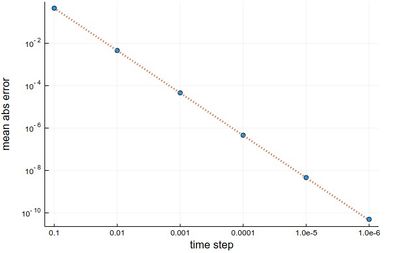
This is more resource intensive but now we get a much better $h^2$ error:

scatter(herror, xlabel="time step", ylabel="mean abs error",
    xticks=(1:6, string.(hlist)), legend=false, yscale=:log10)
plot!(x->100*herror[1]*10.0^-(2x), 1, 6, ls=:dot, lw=3)

We now cover one of the most powerful predictor-corrector algorithms of all, one which is so accurate that most computer algorithms use it as default: the fourth-order Runge-Kutta Method. RK methods are optimized predictor-corrector methods, so they push the idea of Heun's method to the top. The RK4 method finds the optimum correction-prediction (in a way which we do not detail here) to involve these intermediate points:

\begin{align} k_1 &= h\ f(t_n, y_n)\,, \\ k_2 &= h\ f\left(t_n + \frac{h}{2}, y_n + \frac{k_1}{2}\right)\,, \\ k_3 &= h\ f\left(t_n + \frac{h}{2}, y_n + \frac{k_2}{2}\right)\,, \\ k_4 &= h\ f\left(t_n + h, y_n + k_3\right)\,, \end{align}

and then the calculation is explicit:

\begin{align} t_{n+1} &= t_n + h\,, \\ y_{n+1} &= y_n + \tfrac{1}{6}\left(k_1 + 2k_2 + 2k_3 + k_4 \right)\,. \end{align}

In code:

@time for n=1:npts-1
    tn=(n-1)*h-t0;
    k1=h*f(tn,y[n]);
    k2=h*f(tn+(h/2),y[n]+k1/2);
    k3=h*f(tn+(h/2),y[n]+k2/2);
    k4=h*f(tn+h,y[n]+k3);
    y[n+1]=y[n]+(1/6)*(k1+2*k2+2*k3+k4)
end

The error analysis on the same problems as above now yields a very different result:

herror=[];
for h in hlist
    npts=round(Int64,tmax/h);
    y=0.0*collect(1:npts);
    y[1]=-24/37;
    @time for n=1:npts-1
        tn=(n-1)*h;
        k1=h*f(tn,y[n]);
        k2=h*f(tn+(h/2),y[n]+k1/2);
        k3=h*f(tn+(h/2),y[n]+k2/2);
        k4=h*f(tn+h,y[n]+k3);
        y[n+1]=y[n]+(1/6)*(k1+2*k2+2*k3+k4)
    end
    append!(herror,mean(abs.([-(24/37)*cos(3t)-(4/37)*sin(3t) for t in ((1:npts).-1).*h]-y)))
end

  0.006093 seconds (3.91 k allocations: 64.688 KiB)
  0.007069 seconds (41.92 k allocations: 674.766 KiB)
  0.071775 seconds (437.74 k allocations: 6.871 MiB)
  0.805397 seconds (4.40 M allocations: 68.998 MiB, 1.76% gc time)
  6.734973 seconds (43.98 M allocations: 690.260 MiB, 1.41% gc time)
 77.495034 seconds (439.82 M allocations: 6.741 GiB, 1.57% gc time)

scatter(herror, xlabel="time step", ylabel="mean abs error",
    xticks=(1:6, string.(hlist)), legend=false, yscale=:log10)
plot!(x->10^4*herror[1]*10.0^-(4x), 1, 6, ls=:dot, lw=3, ylims=(10^-15,10^-3))

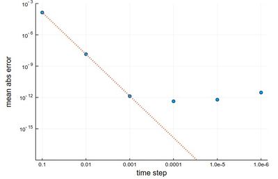
The gain from $h=0.001$ to $h=0.0001$ is marginally better, and for smaller still $h$, it actually becomes worse, due to rounding errors. It works so well that many, if not most, resources would use the RK4 to integrate ODE.

We now turn to the case of coupled equations, in which case the method reads

$$\vec y'=\vec f(t,\vec y)$$

where

$$ \vec y\equiv \begin{pmatrix} y_1\\y_2 \end{pmatrix} \quad\text{and}\quad \vec f\equiv \begin{pmatrix} f_1\\f_2 \end{pmatrix}\,. $$

The methods are the same as before just applying directly to the vectors instead. An interesting coupled system of ODE, namely, the Volterra-Lotka model of prey-predator interactions. This is modelled with the pair of coupled ODE:

\begin{align} \frac{dx}{dt} &= \alpha x - \beta x y, \\ \frac{dy}{dt} &= \delta x y - \gamma y, \end{align}

The functions are implemented as:

function f1(t,y1, y2)
    α*y1-β*y1*y2
end
function f2(t,y1, y2)
    δ*y1*y2-γ*y2
end

Some common initialization for all methods, in particular, we now need two arrays of values to store the evolution of $x$ (in y1) and $y$ (in y2):

tmax=100
h=.001
npts=round(Int,tmax/h)
 
y1=0.0*collect(1:npts);
y2=0.0*collect(1:npts);
 
y1[1]=1;
y2[1]=.1;
 
α=2/3;
β=4/3;
γ=1;
δ=1;

Euler's method in this case reads:

$$\vec y_{n+1}=\vec y_n+h\vec f(t_n,\vec y_n)$$

or, breaking down this equation componentwise:

$$\begin{align} y_{1,n+1}&=y_{1,n}+hf_1(t_n,y_{1,n},y_{2,n})\\ y_{2,n+1}&=y_{2,n}+hf_2(t_n,y_{1,n},y_{2,n}) \end{align}$$

In code:

@time for i=1:npts-1
    y1[i+1]=y1[i]+h*f1((i-1)*h,y1[i],y2[i])
    y2[i+1]=y2[i]+h*f2((i-1)*h,y1[i],y2[i])
end

Heun's version reads:

$$\vec y_{n+1}=\vec y_n+{h\over 2}\left(\vec f(t_n,\vec y_n)+\vec f(t_{n+1},\vec y_n+h\vec f(t_i,\vec y_n)\right)$$

or, breaking down this equation componentwise:

$$\begin{align} y_{1,n+1} &= y_{1,n} + {h\over2} [f(t_n, y_{1,n}, y_{2,n}) + f(t_n + h, y_{1,n} + h f(t_n, y_{1,n}, y_{2,n}), y_{2,n})]\\ y_{2,n+1} &= y_{2,n} + {h\over2} [f(t_n, y_{1,n}, y_{2,n}) + f(t_n + h, y_{1,n}, y_{2,n} + h f(t_n, y_{1,n}, y_{2,n}))] \end{align}$$

In code; where this time we'll find both more convenient and efficient to define auxiliary quantities, that are furthermore invoked more than once:

@time for n=1:npts-1
    tn=(n-1)*h;
    f1left=f1(tn,yH1[n],yH2[n])
    f2left=f2(tn,yH1[n],yH2[n])
    f1right=f1(tn+h,yH1[n]+h*f1left,yH2[n]+h*f2left)
    f2right=f2(tn+h,yH1[n]+h*f1left,yH2[n]+h*f2left)
    yH1[n+1]=yH1[n]+(h/2)*(f1left+f1right)
    yH2[n+1]=yH2[n]+(h/2)*(f2left+f2right)
end

RK4's version reads:

$$ \begin{align} t_{n+1} &= t_n + h\,, \\ \vec y_{n+1} &= \vec y_n + \tfrac{1}{6}\left(\vec k_1 + 2\vec k_2 + 2\vec k_3 + \vec k_4 \right)\,. \end{align} $$

in terms of the intermediate quantities:

$$ \begin{align} \vec k_1 &= h\vec f(t_n, \vec y_n)\,, \\ \vec k_2 &= h\vec f\left(t_n + \frac{h}{2}, \vec y_n + \frac{\vec k_1}{2}\right)\,, \\ \vec k_3 &= h\vec f\left(t_n + \frac{h}{2}, \vec y_n + \frac{\vec k_2}{2}\right)\,, \\ \vec k_4 &= h\vec f\left(t_n + h, \vec y_n + \vec k_3\right)\,, \end{align} $$

In code

@time for n=1:npts-1
    tn=(n-1)*h;
    # Intermediate steps
    k11=h*f1(tn,yRK1[n],yRK2[n]);
    k12=h*f2(tn,yRK1[n],yRK2[n]);
    k21=h*f1(tn+(h/2),yRK1[n]+k11/2,yRK2[n]+k12/2);
    k22=h*f2(tn+(h/2),yRK1[n]+k11/2,yRK2[n]+k12/2);
    k31=h*f1(tn+(h/2),yRK1[n]+k21/2,yRK2[n]+k22/2);
    k32=h*f2(tn+(h/2),yRK1[n]+k21/2,yRK2[n]+k22/2);
    k41=h*f1(tn+h,yRK1[n]+k31,yRK2[n]+k32);
    k42=h*f2(tn+h,yRK1[n]+k31,yRK2[n]+k32);
    # Real step
    yRK1[n+1]=yRK1[n]+(1/6)*(k11+2*k21+2*k31+k41);
    yRK2[n+1]=yRK2[n]+(1/6)*(k12+2*k22+2*k32+k42);
end

Results can be shown in two ways:

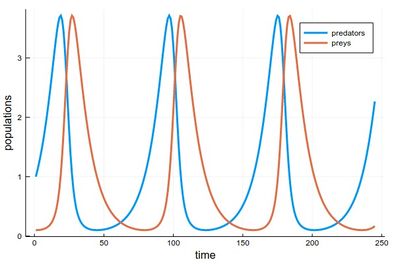
1 - As the respective solutions. This shows the oscillations of predators and preys

pRK=plot([[yRK1[i] for i=1:240], [yRK2[i] for i=1:240]],
lw=3, xlabel="time", ylabel="populations", label="RK4")

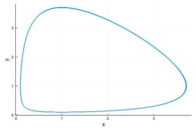
2 - As a phase-space solution, showing the simultaneous state of the system (here, ecosystem), with time as a parametric parameter:

psRK=plot([(yRK1[i], yRK2[i]) for i=1:npts], 
lw=1, xlabel="x", ylabel="y", legend=false)

This comparing the three methods together (the various plots have been evaluated as pE, pH, etc.):

plot(pE,pH,pRK,psE,psH,psRK,layout=(2,3),dpi=150)

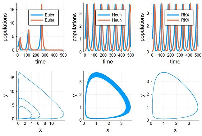
The time-evolutions at the top are over considerably fewer cycles for Heun & RK4 methods than those simulated to produce the phase space solutions, bottom. You can see how the RK4 method stays stable (which is the correct behaviour) while the Heun method slowly drifts towards the stable point.

— • 16:24, 8 March 2021

@@ Line 48: / Line 48: @@
 The first version can plot over the range 0–4 but does so by not plotting the full function, while the second (with x-steps of 0.0001 allowing for the nice curvature) shows everything but would return an error if going over the limit where the argument gets negative.
-So much for integration. How about the reverse process, i.e., derivation. We can use the diff command that computes finite differences:
+So much for integration.
-<syntaxhighlight lang="python">
-diff(1:.5:10)
-</syntaxhighlight>
-returns an array of 18 elements, all equal to 0.5. In this way, it is easy to compute a finite-difference derivative:
-<syntaxhighlight lang="python">
-plot(diff([sin(pi*x) for x=0:.01:1])./.01)
-</syntaxhighlight>
-This is a cosine. Importantly for numerical methods, one should look for simple tricks that maximise numerical accuracies. The idea behind differentiation comes from Taylor expansion:
-\begin{equation}
-\label{eq:taylorf}
-f(x\pm\epsilon)=f(x)\pm\epsilon f'(x)+{\epsilon^2\over2} f''(x)\pm{\epsilon^3\over6} f'''(x)+o(\epsilon^4)
-\end{equation}
-that we wrote for both $\pm\epsilon$, and using the $o$-notation to mean that terms we neglected are of the order of $\epsilon^4$. From this, one can get an obvious numerical approximation for the derivative
-$$f'(x)\approx{f(x\pm\epsilon)-f(x)\over\epsilon}+o(\epsilon)$$
-meaning we can expect an error of the order of $\epsilon$ with this method. Observe however how one can sneakily cancel the $\epsilon^2$ term from \eqref{eq:taylorf} by subtracting $f(x-\epsilon)$ from $f(x+\epsilon)$:
-$$f(x+\epsilon)-f(x-\epsilon)=2\epsilon f'(x)+{\epsilon^3\over 3}{f'''(x)}+o(\epsilon^4)$$
-so that we have a much better approximation by computing with this slight variation:
-$$f'(x)={f(x+\epsilon)-f(x-\epsilon)\over 2\epsilon}+o(\epsilon^2)$$
-since $\epsilon^2\ll\epsilon$. The computational cost is the same, the numerical gain is considerable. Let's write a function. We'll it call <tt>Dl</tt> for "Differentiate list":
-<syntaxhighlight lang="python">
-function Dl(f, δx, method="central")
-    if method=="left"
-        diff(f)/δx
-    elseif method=="central"
-        [f[i+1]-f[i-1] for i=2:length(f)-1]/(2*δx)
-    end
-end
-</syntaxhighlight>
-Let us compare the two methods for
-<syntaxhighlight lang="python">
-δx=0.1;
-mysin=[sin(pi*x) for x in 0:δx:1]
-</syntaxhighlight>
-We find fairly identical-looking results:
-<syntaxhighlight lang="python">
-plot([Dl(mysin,δx,"central"), Dl(mysin,δx,"left")], legend=false)
-</syntaxhighlight>
-<center><wz tip="The cosine according to the central and forward (left) finite-difference methods. A small error is visible in the center.">[[File:Screenshot_21-02-2020_193810.jpg|400px]]</wz></center>
-This error is actually quite large if looked at properly: (note the comparison to lists of different size, the central method removes two points)
-<syntaxhighlight lang="python">
-plot([
-        Dl(mysin,δx,"central")-[pi*cos(pi*i) for i in δx:δx:1-δx],
-        Dl(mysin,δx,"left")-[pi*cos(pi*i) for i in 0:δx:1-δx]
-    ], legendtitle="Method", legend=:bottomleft, label=["central" "left"])
-</syntaxhighlight>
-<center><wz tip="Errors between the two differentiation methods when comparing to the exact result.">[[File:Screenshot_21-02-2020_194041.jpg|400px]]</wz></center>
-This idea (and method) can be further exploited. By working out how to cancel the next-order terms, we arrive at the so-called [https://en.wikipedia.org/wiki/Five-point_stencil Five-point stencil]:
-$$f'(x) \approx \frac{-f(x+2\epsilon)+8 f(x+\epsilon)-8 f(x-\epsilon)+f(x-2\epsilon)}{12\epsilon}$$
-which we can add to our function:
-<syntaxhighlight lang="python">
-function Dl(f, δx, method="central")
-    if method=="left"
-        diff(f)/δx
-    elseif method=="central"
-        [f[i+1]-f[i-1] for i=2:length(f)-1]/(2*δx)
-    elseif method=="fivepoints"
-        [-f[i+2]+8f[i+1]-8f[i-1]+f[i-2] for i=3:length(f)-2]/(12*δx)
-    end
-end
-</syntaxhighlight>
-Comparing their errors:
-<syntaxhighlight lang="python">
-plot([
-        Dl(mysin,δx,"fivepoints")-[pi*cos(pi*i) for i in 2δx:δx:1-2δx],
-        Dl(mysin,δx,"central")-[pi*cos(pi*i) for i in δx:δx:1-δx],
-        Dl(mysin,δx,"left")-[pi*cos(pi*i) for i in 0:δx:1-δx]
-    ], legendtitle="Method", legend=:bottom,
-       label=["5 points" "central" "left"], ylims=(-.005,.001))
-</syntaxhighlight>
-<center><wz tip="Errors between the three differentiation methods when comparing to the exact result. Note how the finite difference exploses out of the plotting range.">[[File:Screenshot_21-02-2020_195518.jpg|400px]]</wz></center>
-If we want a more quantitative study at the errors, we can look at how it scales for various $\epsilon$. This will allow us to look at logarithmic steps:
-<syntaxhighlight lang="python">
-lδx=[10.0^(-k) for k in 1:7]
-err1=[mean(abs.(Dl([sin(pi*x) for x in 0:δx:1], δx, "left")-[pi*cos(pi*x) for x in 0:δx:1-δx])) for δx in lδx]
-err2=[mean(abs.(Dl([sin(pi*x) for x in 0:δx:1], δx, "central")-[pi*cos(pi*x) for x in δx:δx:1-δx])) for δx in lδx]
-err3=[mean(abs.(Dl([sin(pi*x) for x in 0:δx:1], δx, "fivepoints")-[pi*cos(pi*x) for x in 2δx:δx:1-2δx])) for δx in lδx]
-plot([abs.(err1) abs.(err2) abs.(err3)],
-    yscale=:log10, label=["left" "central" "5 points"],
-    xlabel="10^-k step", ylabel="Mean abs error", lc=[:red :blue :green])
-plot!([x->10.0^(-x) x->10.0^(-2x) x->10.0^(-4x)],1,7,
-yscale=:log10, ylims=(10^(-15),1), lc=[:red :blue :green], ls=:dash, label=["" "" ""])
-</syntaxhighlight>
-with the beautiful result:
-<center><wz tip="The fight between rounding error and numerical approximation. Sometimes ''le mieux est l'ennemi du bien''. In dashed the theoretical slope in the timestep.">[[File:Screenshot_21-02-2020_205530.jpg|400px]]</wz></center>
-As one can see, the best method worsens for $\epsilon<10^{-4}$ so it will actually work better (and faster) for not too small an $\epsilon$.
 <span id="newtonraphson">Let us now</span> turn to another typical numerical method: a root-finding algorithm. We used a so-called [https://en.wikipedia.org/wiki/Bisection_method bisection method] previously when generating our own random numbers, which is easy to implement but not very efficient. A simple but good improvement is the [https://en.wikipedia.org/wiki/Newton%27s_method Newton–Raphson method] ([[Newton]] used it for the particular case of polynomials; Raphson extended it to arbitrary functions). The idea is to start with a blind guess $x_0$ around the solution and replace the real function $f(x)$ by a linear approximation with the same slope at $x_0$, i.e., $h(x)=f'(x_0)x+\beta$ with $\beta$ such that $h(x_0)=f(x_0)$ which yields