Crash Course in Scientific Computing

XIV. Integrals

We will now start to apply algorithms, or precise recipes, to numerical problems. We will start with a simple one, that has a clear physical interpretation: integration of 1D functions of one variable, i.e., the computation of areas. We will also look at a precise application of such computations (which are of interest on their own, of course). Namely, we will look at how to generate more efficiently 1D random numbers on our own, that is, following any given probability distribution (a positive, normalized function). For instance, let us say we want to simulate the ground state of a particle in a box, with probability distribution over $[0,1]$ given by:

$$\psi^2(x)=2\sin^2(\pi x)$$

We remind that one can use unicode characters (by entering \psi+TAB) to call our density of probability ψ2, which in quantum mechanics is given by the modulus square of the probability amplitude (in 1D the wavefunction can always be taken real so we do not need worry about the modulus):

ψ2(x)=2*sin(pi*x)^2

That's our density of probability:

using LaTeXStrings
default(; w=3)
plot(ψ2,0,1, title=L"2\sin^2(x)", xlabel=L"x", ylabel=L"\psi^2(x)",dpi=150,legend=false)

where we decorated the plot with a lot of options, but the width which we gave as a default attribute, not to do it in the future (and since we like thick lines).

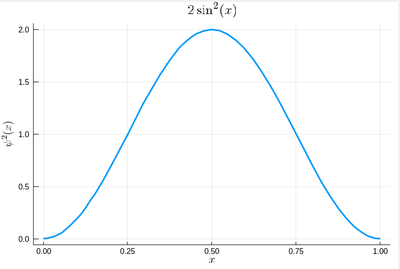
We have already seen a simple method to draw random numbers that follow such a probability distribution but this was fairly inefficient. We now implement a technique, known as inverse transform sampling, which will return a valid point every time. To do that, we need to compute quantities such as $F(y)\equiv\int_0^y\psi^2(x)\,dx$, or the so-called cumulative. Of course, we should find that $F(1)=1$ (normalization condition), so we can check that as well. The simplest way to compute such integrals numerically is to bring to the computer the mathematical definition we have given of the integral, namely, in terms of Riemann sums, i.e., as a sum of parallelograms defined on a partition of the support of the function (here $[0,1]$) cut into $n$ intervals. Calling $f$ the function to integrate, this is defined as:

$$R_n=\sum_{i=1}^{n}f(x_i)\delta(i)$$

a, b = 0, 1; # boundaries
lx=range(a, stop=b, length=11) # list of x intervals
δ=diff(lx) # widths of intervals
lxi=lx[1:end-1] # x_i points of parallelograms

We can now compute our integral over the entire interval to check the normalization:

sum([ψ2(lxi[i])*δ[i] for i=1:length(lxi)])

1.0

The cumulative is itself obtained as:

Ψ=[sum([ψ2(lxi[i])*δ[i] for i=1:j]) for j=1:length(lxi)]

This is the result for 100 intervals (length=101 above):

plot(lxi, Ψ, legend=false, title="Cumulative")

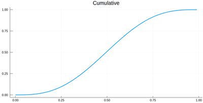
Now the generation of a random number following the initial distribution works as follows. We select randomly (uniformly) a number on the $y$-axis of the cumulative and find the corresponding $x$ such that $F(x)=y$. Those $x$ are $f$ distributed.

This can be simply achieved as follows (later we'll see a more sophisticated way but let's just use the most straightforward way to get to the point):

yr=rand()
fx=lx[[findmin(abs.(Ψ.-rand()))[2] for i=1:10]]

Here are some positions where our ground state collapsed:

10-element Array{Float64,1}:
 0.55
 0.96
 0.24
 0.5 
 0.58
 0.16
 0.67
 0.74
 0.08
 0.46

histogram(lx[[findmin(abs.(Ψ.-rand()))[2] for i=1:10^7]], bins=0:.01:1,norm=true)

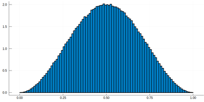
Note that the binning cannot be less than the $\delta$ step, otherwise we will get "holes" (and also the wrong normalization) (?!)Too fine binning, resulting in holes and wrong normalization.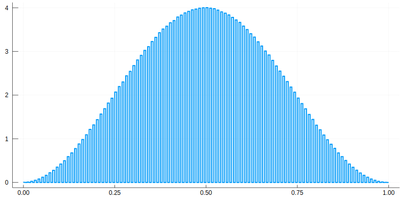
.

Compare the efficiency of inverse transform sampling against rejection sampling.

Write a code to sample the probability density functions for the 1D quantum harmonic oscillator. Make an animation showing simultaneous Monte-Carlo sampling of the first 5 states of the system, displaying sampled positions on the $x$ axis and the energy on the $y$ axis. Implement an option to fade gradually previous points as the animation progresses.

Putting our results together in a (clumsy) function of our own:

# Riemann sums of f with n intervals in [0, 1]
function myRiemann(f, n)
    a, b = 0, 1; # boundaries
    lx=range(a, stop=b, length=n) # list of x intervals
    δ=diff(lx); # widths of intervals
    lxi=lx[1:end-1]; # x_i points of parallelograms
    sum([f(lxi[i])*δ[i] for i=1:length(lxi)])
end

Then we can try:

myRiemann(exp, 10^3)

1.717421971020861

The result is fairly close to the exact

$$e-1\approx1.718281828459045\tag{1}$$

However we'll find that our method is fairly limited since it requires a lot of intervals (a million) to achieve a fairly modest accuracy (6 digits):

scatter([abs(myRiemann(exp, 10^i)-(exp(1)-1)) for i=1:6], yscale=:log10,
         ylabel="error", xlabel=L"\hbox{Number of points } 10^x", 
         label="Riemann sum", dpi=200)

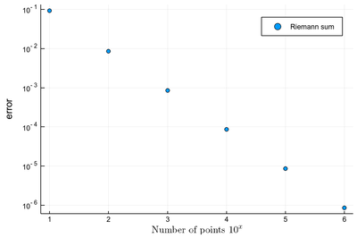
It is the purpose of numerical methods to learn how to use algorithms that are efficient, in the sense that they are accurate, fast and resource-effective.

It is easy to be brutal and terribly inefficient with a computer. In fact a fairly trivial enhancement of our method leads to considerable improvement. We have used Riemann integrals by taking the leftmost point. We could also take the rightmost point, or the central point, i.e., their average:

function myRiemann(f, n, method="mid")
    a, b = 0, 1; # boundaries
    lx=range(a, stop=b, length=n) # list of x intervals
    δ=diff(lx); # widths of intervals
    if method == "left"
        lxi=lx[1:end-1]; # x_i points of parallelograms
    elseif method == "right"
        lxi=lx[2:end];
    else
        lxi=(lx[1:end-1]+lx[2:end])/2;
    end
    sum([f(lxi[i])*δ[i] for i=1:length(lxi)])
end

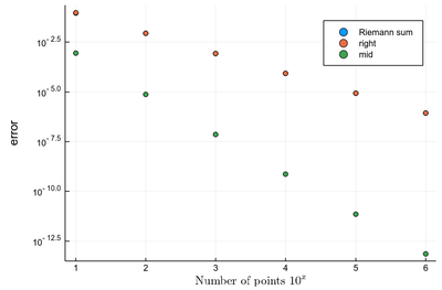
There is a huge gain in precision by evaluating the function elsewhere? Why? Clearly because we find a compensation of errors. Note that evaluating at the central point is equivalent to computing the area of a trapezoid, which also explain why the area is better estimated. For this reason, this method of integration is called the "trapezoidal rule".

Can it be further improved? Of course, following the same idea, one could approximate the function not by a straight line, but by a curve. Polynomials make easy curves and they are easy to integrate too, not even numerically, but symbolically. That brings forward the so-called "Newton-Cotes quadrature" that specify the weights $\omega_i$ and the locations $x_i$ where to sample the function to integrate:

$$\int _{a}^{b}f(x)\,dx\approx \sum _{i=0}^{n}w_{i}\,f(x_{i})$$

Using the Lagrange interpolating polynomials that we have previously introduced, we can interpolate with two points (a line), at $x_1$ and $x_2=x_1+h$. The Lagrange basis in this case reads:

\begin{align} l_1(x)&={x-x_2\over x_1-x_2}\\ l_2(x)&={x-x_2\over x_2-x_1} \end{align}

and the interpolating Lagrange polynomial becomes:

$$P_f(x)=f_1l_1(x)+f_2l_2(x)$$

where $f_i\equiv f(x_i)$, which simplifies to (collecting $x$ and substituting $h=x_2-x_1$):

$$P_f(x)=x{f_2-f_1\over h}+(f_1+{x_1\over h}f_1-{x_1\over h}f_2)$$

So the integral can be found by performing it symbolically on the polynomials (which are easy to integrate exactly) and turn the problem into mere additions of weighted values of the functions at given points (quadrature):

\begin{align} \int_{x_1}^{x_2}f(x)\,dx&\approx\int_{x_1}^{x_2}P_f(x)\,dx\\ &={f_2-f_1\over h}\left.{x^2\over 2}\right|_{x_1}^{x_1+h}+(f_1+{x_1\over h}f_1-{x_1\over h}f_2)x\left.\vphantom{x^2\over2}\right|_{x_1}^{x_1+h}\\ &={f_1+f_2\over 2h} \end{align}

and we recover the trapezoidal rule.

With three points, at $x_1$, $x_2=x_1+h$ and $x_3=x_1+2h$, the Lagrange polynomials read:

\begin{align} l_1(x)&={x-x_2\over x_1-x_2}{x-x_3\over x_1-x_3}\\ l_2(x)&={x-x_1\over x_2-x_1}{x-x_3\over x_2-x_3}\\ l_3(x)&={x-x_1\over x_3-x_1}{x-x_2\over x_3-x_2} \end{align}

and the Lagrange interpolating polynomial:

$$P_f(x)=f_1l_1(x)+f_2l_2(x)+f_3l_3(x)$$

simplifies to:

$$ {f_1\over 2h^2}(x^2-x(x_2+x_3)+x_2x_3) -{f_2\over h^2}(x^2-x(x_1+x_3)+x_1x_3) +{f_3\over 2h^2}(x^2-x(x_1+x_2)+x_1x_2) $$

Now one can integrate each polynomial in turn. We work out the one that goes with the term $f_1$ (others follow similarly):

\begin{align} \int_{x_1}^{x_1+2h}&(x^2-x(x_2+x_3)+x_2x_3)\,dx={}\\ &{(x_1+2h)^3-x_1^3\over 3}-{(x_1+2h)^2-x_1^2\over 2}(x_2+x_3)+((x_1+2h)-x_1)x_2x_3\\ &={6x_1^2h+12x_1h^2+8h^3\over 3}-{4x_1h+4h^2\over 2}(2x_1+3h)+2h(x_1^2+3x_1h+2h^2)\\ &={2\over 3}h^3 \end{align}

So, incredibly, there is massive simplifications and one is left with a simple ${f_1\over2h^2}\times{2\over 3}h^3=f_1{h\over 3}$ expression meaning a $h/3$ weighting of the first sampled point. We let you compute the other coefficients yourself:

Show that simplifications of the integrated Lagrange polynomials result in the simple quadrature formula for a cubic (or three-points) integration of $f$:

$$\int_{x_1}^{x_3}P_f(x)\,dx={h\over 3}(f_1+4f_2+f_3)\,.\tag{2}$$

The following piece of code implements the 3-points ($n=3$) Newton Cotes method:

# Integrate f between a and b with a n-point method:
function NewtonCotes(f, a, b, n=3)
    h=(b-a)/n
    if n==3
        (h/3)*(f(a)+4f((a+b)/2)+f(b))
    else
        println("Sorry, $(n)-point method is not available.")
    end
end
 
julia> NewtonCotes(exp,0,1)
1.7188611518765928

so quite accurate by using 3 points only (the exact result is Eq. (1))! To increase accuracy one can do two things, increase $n$, or break the functions into smaller intervals and iterate the method. The latter is natural in spirit as extending the Riemann idea to Lagrange-interpolated functions. This is called a "composite Newton-Cotes method" and can be implemented either through computer-assisted iteration:

julia> δx=.1
0.1
 
julia> sum([NewtonCotes(exp,i,i+δx) for i=0:δx:1-δx])
1.7182818881038564

or one can provide directly the expression that sums the Newton Cotes formula on each subinterval, e.g.,

$${\displaystyle {\begin{aligned}\int _{a}^{b}f(x)\,dx&\approx {\frac {h}{3}}\sum _{j=1}^{n/2}{\bigg [}f(x_{2j-2})+4f(x_{2j-1})+f(x_{2j}){\bigg ]}\\{}&={\frac {h}{3}}{\bigg [}f(x_{0})+2\sum _{j=1}^{n/2-1}f(x_{2j})+4\sum _{j=1}^{n/2}f(x_{2j-1})+f(x_{n}){\bigg ]},\tag{3}\end{aligned}}}$$

where $x_j=a+jh$ for $0\le j\le n$ with $h=(b-a)/n$.

Prove Eq. (3).

This is the error made with this 3-point method:

lϵ=abs.([sum([NewtonCotes(exp,i,i+δx) for i=0:δx:1-δx])-(exp(1)-1) for δx in lδx])
6-element Array{Float64,1}:
 5.964481131215393e-8  
 5.9676708019651414e-12
 2.220446049250313e-15 
 1.7186252421197423e-13
 4.369393735714766e-12 
 2.1261659099991448e-11
 
plot(lϵ, yscale=:log10, label="3-point Newton Cotes")
scatter!(lϵ, yscale=:log10, label=false, xlabel=L"h=10^{-k}", ylabel="error", dpi=300)

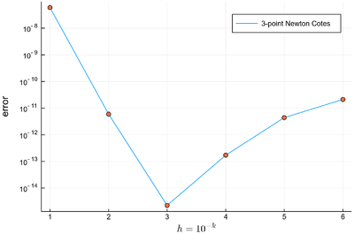
Interestingly, increasing the number of points actually increase the error, so trying to get a better result by assigning more resources is not a guaranteed better strategy. This is due to numerical errors from the larger number of operations involved, overcoming the benefits of a finer grid of integration. We will come back to this phenomenon below. For now, we will refine the method by improving the quality of the interpolation by extended to higher-orders of interpolations, that is, with more points in the interval. Possibly the most famous formula is the Simpson 3/8 rule which is a healthy practice in awkward (but easy) algebra to bring to its conclusion to find that:

Show that the 4-point interpolation provides the (so-called Simpson's 3/8) rule:

$$\int_{x_1}^{x_4} P_f(x)\,dx={\displaystyle {\frac {3h}{8}}(f_{0}+3f_{1}+3f_{2}+f_{3})}$$

where $f_i\equiv f(x_1+ih)$ with step $h\equiv(x_4-x_1)/3$ for $1\le i\le 3$.

This is better than the 3-point method but still of order $h^5$. To go to order $h^7$ one needs Boole's rule which reads:

$$\int_{x_1}^{x^5}P_f(x)\,dx={\displaystyle {\frac {2h}{45}}(7f_{0}+32f_{1}+12f_{2}+32f_{3}+7f_{4})}$$

with the same definitions as above (now $h\equiv(x_5-x_1)/4$) and that you could similarly demonstrate, if interested. You can also find the cases elsewhere (e.g., here or here). Here is an implementation of cases up to 7-point integration:

function NewtonCotes(f, a, b, n=4)
    h=(b-a)/(n-1)
    if n==2
        (h/2)*(f(a)+f(b))
    elseif n==3
        (h/3)*(f(a)+4f(a+h)+f(b))
    elseif n==4
        (3h/8)*(f(a)+3f(a+h)+3f(a+2h)+f(b))
    elseif n==5
        (2h/45)*(7f(a)+32f(a+h)+12f(a+2h)+32f(a+3h)+7f(a+4h))
    elseif n==6
        (5h/288)*(19f(a)+75f(a+h)+50f(a+2h)+50f(a+3h)+75f(a+4h)+19f(a+5h))
    elseif n==7
        (h/140)*(41f(a)+216f(a+h)+27f(a+2h)+272f(a+3h)+27f(a+4h)+216f(a+5h)+41f(a+6h))
    else
        println("Sorry, $(n)-point method is not available.")
    end
end

which it is now easy to benchmark by compositing the function over steps of smaller sizes, e.g.:

julia> lδx=[2.0^(-k) for k=1:16]
16-element Array{Float64,1}:
 0.5             
 0.25            
 0.125           
 0.0625          
 0.03125         
 0.015625        
 0.0078125       
 0.00390625      
 0.001953125     
 0.0009765625    
 0.00048828125   
 0.000244140625  
 0.0001220703125 
 6.103515625e-5  
 3.0517578125e-5 
 1.52587890625e-5

which gives us for $\int_0^1 e^x\,dx$:

p=plot();
for n=2:7
    lϵ=filter(!iszero, abs.([sum([NewtonCotes(exp,i,i+δx,n) for i=0:δx:1-δx])-(exp(1)-1) for δx in lδx]));
    plot!(lϵ, yscale=:log10, label="$(n)-point")
    scatter!(lϵ, label=false, c=:red, m=2)
end
plot!(xticks = (1:length(lδx), ["\$2^{-$(k)}\$" for k∈1:length(lδx)]), dpi=200,
      xformatter = :latex, xlabel = "Step in composite Newton Cotes", ylabel="Error")

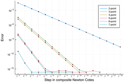
Error in the various $n$-point Newton Cotes composite integrations on $\int_0^1e^x\,dx$. The machine precision is $\approx 10^{-16}$. Points not shown mean that the error is zero.

The higher-order method quickly reach machine precision and thus cannot be more accurate: this is a limitation of the computer, not of the method itself. When points are not shown, this is because the result is exactly the same as found by exp(1)-1 from the computer, and one cannot hope for a better result than this one (with machine precision). So we have basically achieved (numerical) perfection!

Coming back to the mysterious feature noted previously, that a better integration-step was making the integration worse, we can see from the above that this was caused by numerical error linked to the use of the unnatural (to the computer) basis 10. If we use the base 2 instead, one stays clamped to the machine eps() when not converging to the (Float64) exact result. This is how our previous result compares to the basis 2 one:

lϵ10=abs.([sum([NewtonCotes(exp,i,i+δx,3) for i=0:δx:1-δx])-(exp(1)-1) for δx in lδx10]);
lϵ2=abs.([sum([NewtonCotes(exp,i,i+δx,3) for i=0:δx:1-δx])-(exp(1)-1) for δx in lδx2]);
 
closeall()
plot((lδx10, lϵ10), label="Base 10", lw=2, yscale=:log10, xscale=:log10, xflip=true)
scatter!((lδx10, lϵ10), yscale=:log10, xscale=:log10, xflip=true, c=:blue, m=3, label=false)
plot!((lδx2[notzero], lϵ2[notzero]), label="Base 2", yscale=:log10, xscale=:log10, xflip=true, lc=:red)
scatter!((lδx2[notzero], lϵ2[notzero]), yscale=:log10, xscale=:log10, xflip=true, c=:red, m=2, label=false)
plot!(xlabel="Integration step", ylabel="Error", title="3-point Newton Cotes integration", xflip=true, dpi=200)

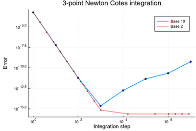
This plot has, on its own, some interesting features, including using different points on the $x$-axis and a representation compatible to that we used so far: right on the $x$ axis meaning better, not smaller (xflip).

We could, finally (we should), pack-up our code in a built-in, well-documented function. Here is a minimal attempt at that:

# Integrate f from a to b with an n-point composite Newton-Cotes method of step δx.
# e.g., julia> MyIntegral(cos, 0, pi/2, 2^-24)
# 0.9999999999999999
function MyIntegral(f, a, b, δx=2^-10, n=4)
    if a > b
        -1*MyIntegral(f, b, a, δx, n)
    elseif a==b
        0
    else
        sum([NewtonCotes(f,i,i+δx,n) for i=a:δx:b-δx])
    end
end

Of course, other people already wrote such functions, which hopefully have been designed with much more care and robustness for all possible situation, and that are available through packages. For numerical integration of 1D functions, one can use QuadGK which is based on the so-called Gauss–Kronrod quadrature formula, which basically figures out how to best choose the points $x_i$ and how to weight them:

using QuadGK
@time quadgk(exp, 0, 1)

The result is both pretty fast and accurate:

  0.000034 seconds (9 allocations: 304 bytes)
(1.718281828459045, 0.0)

Note that it also returns an estimate of the absolute error (second term, here, 0). In comparison, our implementation looks quite efficient in terms of accuracy and speed:

julia> [@time MyIntegral(exp, 0, 1, 2^-10, n) for n∈2:7]
  0.000042 seconds (8 allocations: 8.469 KiB)
  0.000080 seconds (8 allocations: 8.469 KiB)
  0.000106 seconds (8 allocations: 8.469 KiB)
  0.000124 seconds (8 allocations: 8.469 KiB)
  0.000134 seconds (8 allocations: 8.469 KiB)
  0.000115 seconds (8 allocations: 8.469 KiB)
6-element Array{Float64,1}:
 1.7182819650158139
 1.7182818284590458
 1.7182818284590453
 1.7182818284590453
 1.7182818284590453
 1.718281828459045

but this was on this one easy case (the exponential between 0 and 1). More complicated functions will cause difficulties for all methods, which the implemented versions will be more robust against:

julia> @time quadgk(cos, 0, 10*pi)
  0.430831 seconds (6.67 M allocations: 131.071 MiB, 11.72% gc time)
(-1.5511618370825867e-14, 1.5331823026708485e-19)

In comparison to this, our implementation reveals its limitations both in terms of speed, memory and accuracy:

julia> [@time MyIntegral(cos, 0, 10*pi, 2^-24, n) for n∈2:7]
 16.153582 seconds (9 allocations: 3.927 GiB, 0.07% gc time)
 21.565125 seconds (9 allocations: 3.927 GiB, 0.75% gc time)
 26.902072 seconds (9 allocations: 3.927 GiB, 0.60% gc time)
 32.140675 seconds (9 allocations: 3.927 GiB, 0.40% gc time)
 37.336019 seconds (9 allocations: 3.927 GiB, 0.33% gc time)
 42.890000 seconds (9 allocations: 3.927 GiB, 0.29% gc time)
6-element Array{Float64,1}:
 -1.984187081305322e-8 
 -1.9841871368164732e-8
 -1.984187125714243e-8 
 -1.984187170123164e-8 
 -1.9841871812253942e-8
 -1.9841871812253942e-8

Interestingly, the Newton Cotes method various orders do not improve on the accuracy! This is something unexpected which is worth further study.

Study the error of the various Newton Cotes methods on other functions and other intervals.

One can implement the following function:

function convergenceNC(f, a, b, exact)
    closeall;
    p=plot();
    lδx=[2.0^(-k) for k=1:16]
    for n=2:7
        plot!(filter(!iszero,[abs.(MyIntegral(f,a,b,δx,n)-exact) for δx in lδx]), yscale=:log10)
    end
    p
end

and try it on various functions and ranges, e.g.,

convergenceNC(exp, 0, 1, exp(1)-1)
convergenceNC(sqrt, 0, 1, 2/3)
convergenceNC(sin, 0, pi, 2)
convergenceNC(cos, 0, pi, 0)
convergenceNC(x->sin(x)^2, 0, pi, pi/2)
convergenceNC(x->exp(-x^2), 0, 1, pi/2)

the latter case will require

using SpecialFunctions

We find that trigonometric functions are not sensible to the order of the Newton-Cotes integration, that functions like $\sqrt{\phantom{x}}$ are but not in the slope, merely as their abscissa, and that functions involving exponential change their slopes as expected. The reason for this behaviour is not known to me and should be investigated (looking at the Lagrange decomposition and exact quadrature results).