Crash Course in Scientific Computing
XIII. Root Finding
We have seen in the previous lecture as one of the earliest algorithm ever devised the one to compute the square root of 2. Looked at in a more general fashion, what this algorithm achieves is the particular case of a central problem of Mathematics: solving an equation. Namely, in this case:
$$f(x)=0\label{eq:eq}$$
where $f(x)=x^2-2$. Nowadays, by completion of the square, we would solve Eq. \eqref{eq:eq} by writing it as $(x-\sqrt{2})(x+\sqrt{2})=0$ but this does not, actually, give us the numerical value. A computer would do this with a so-called root-finding algorithm. The simplest one is just a brute force approach where we compute all the values on a finite grid and take the closest one to the sought result. We can build the algorithm by steps:
# define a grid of trial points
δx=0.1;
lx=0:δx:2;

# Evaluate the function on this grid:
julia> (x->x^2-2).(lx)
21-element Array{Float64,1}:
 -2.0
 -1.99
 -1.96
 -1.91
 -1.8399999999999999
 -1.75
 -1.6400000000000001
 -1.51
 -1.3599999999999999
 -1.19
 -1.0
 -0.7899999999999998
 -0.56
 -0.30999999999999983
 -0.04000000000000026
  0.25
  0.5600000000000005
  0.8899999999999997
  1.2400000000000002
  1.6099999999999999
  2.0

# take the positive values:
abs.((x->x^2-2).(lx));

# find the smallest number (i.e., closest to zero):
julia> findmin(abs.((x->x^2-2).(lx)))
(0.04000000000000026, 15)
The smallest number is 0.04000000000000026, which is not very close to zero (only to within the first two digits), but that is not surprising given the coarse grid of points we took. This is obtained at the 15th index, so our approximate solution is:
julia> lx[findmin(abs.((x->x^2-2).(lx)))[2]]
1.4
which is not too bad for a wild guess:
julia> 1.4*1.4
1.9599999999999997

julia> 1.5*1.5
2.25
We can embed this "algorithm" into a (poor man's) root-find function:
# find x such that f(x)=0 in [a, b] with accuracy δx
function myfindroot(f, a, b, δx)
    lx=a:δx:b;
    lx[findmin(abs.((x->x^2-2).(lx)))[2]]
end
in which case we can, painfully, try to improve our accuracy. We know that the root was between the 15th and 16th element of our grid, so we can focus our search there:
julia> for k=2:10
        @time println(myfindroot(x->x^2-2, lx[15], lx[16], 10.0^-k))
       end
1.41
  0.000031 seconds (17 allocations: 544 bytes)
1.414
  0.000016 seconds (17 allocations: 1.234 KiB)
1.4142
  0.000021 seconds (17 allocations: 8.359 KiB)
1.41421
  0.000068 seconds (18 allocations: 78.625 KiB)
1.414214
  0.000772 seconds (18 allocations: 781.750 KiB)
1.4142136
  0.008025 seconds (18 allocations: 7.630 MiB)
1.4142135599999999
  0.153763 seconds (18 allocations: 76.294 MiB, 47.71% gc time)
1.4142135619999998
  0.839739 seconds (18 allocations: 762.940 MiB, 5.92% gc time)
Killed
That seems to work but the time, and eventually the resources, required crashed the machine. The problem is of course the number of points that we compute each time:
julia> length(2:10.0^-10:10)
80000000001
That's 80 billions, which is an overkill, when we only need to know the functions on the points close to root itself, not the whole range that extends far from it. The above implementation is an example of a working but inefficient, brute-force method that should be avoided. An algorithm should strive to optimize times and resources, and both if possible. A considerable improvement would be to return the interval surrounding the root for sure and focus our search there. This can be done by returning not our best estimates of the zero but its surrounding values, so that we can enclose both the root (and our best estimate of it):
function myfindroot(f, a, b, δx)
    lx=a:δx:b;
    x0=findmin(abs.(f.(lx)))[2]
    [lx[x0-1], lx[x0+1]]
end
Now this is immediate (a @time would show 0.000017 seconds (13 allocations: 656 bytes) for all entries!) and quickly converges to the result within machine precision:
julia> xmin=0; xmax=2;
       for k=1:16
           global xmin, xmax = myfindroot(x->x^2-2, xmin, xmax, 10.0^-k)
           println("$((xmin+xmax)/2)\t\t\t$(((xmin+xmax)/2)-sqrt(2))")
       end
1.4                     -0.014213562373095234
1.41                    -0.004213562373095225
1.4140000000000001      -0.0002135623730949998
1.4142                  -1.3562373095243885e-5
1.41421                 -3.5623730951783728e-6
1.4142139999999999      4.376269047146053e-7
1.4142136               3.762690492514764e-8
1.4142135599999999      -2.3730952758427293e-9
1.414213562             -3.730951103619873e-10
1.4142135624            2.690492273416112e-11
1.41421356237           -3.0950797480500114e-12
1.4142135623729999      -9.525713551283843e-14
1.4142135623731         4.884981308350689e-15
1.41421356237309        -5.10702591327572e-15
1.414213562373095       -2.220446049250313e-16
1.414213562373095       -2.220446049250313e-16
Compare to:
julia> sqrt(2)
1.4142135623730951
The error is that our method gives 1.4142135623730950 (last 0 added explictely) while the computer machine has 1.4142135623730951 so the difference is the last floating-point digit, which is eps() or -2.220446049250313e-16. Note that to within 22 decimals, the actual value is 1.4142135623730950488 so our result turns out to be in fact more accurate! While this is true in absolute precision, this doesn't matter in machine precision:
julia> 2-1.4142135623730951^2
-4.440892098500626e-16

julia> 2-1.4142135623730950^2
4.440892098500626e-16
Does it mean that we have completed our task of root-finding? This is, for instance, the seventh-root of three:
julia> xmin, xmax = 0, 2
for k=1:16
    global xmin, xmax = myfindroot(x->x^7-3, xmin, xmax, 10.0^-k)
end

julia> (xmin+xmax)/2
1.169930812758687

julia> (ans^7)
3.000000000000001
In fact, even this modest improvement, that spares us the computation of billions of useless points, is still very far from optimum, as we still compute the same number of points in each iterated loop, namely, that of our initial grid (since we divide the step by ten and apply it to one interval). So we, technically, still overcompute over a number of points that are not needed. Fixing this is not very complicated. Basically, we would just need to start with a minimal grid, which with our trick of surrounding the best guess, means three. In fact, one need only two points. That gives rise to the so-called bisection method which relies, for a continuous function, on the fact that on both sides of a "root", or "zero" (these are synonyms for "solution") of the equation, it has to change sign (assuming it is, of course, continuous). Therefore, one can halve the current interval in half and look for which one maintains this property: that is the one that contains the root. It could be that both feature this property, in which case one has at least three roots. A typical difficulty in finding roots is to finding all of them, in which case it helps considerably if we know how many of them we are looking for. On the other hand, we know the result we are looking for (zero), so we can keep looking until we reach the lowest possible accuracy, which is not compulsorily the machine epsilon. This is a possible julia implementation, where we stop if the algorithm didn't converge after some number of iterations (100 by default):
function bisection(f, a, b, maxit=100)
    c=(a+b)/2
    it=0
    while abs(f(c))>0 && it<maxit
        println("a=$(a)\t\t c=$(c)\t\t b=$(b)")
        println("f(a)=$(f(a))\t f(c)=$(f(c))\t f(b)=$(f(b))\n")
        if f(a)*f(c)<0
            b=c;
        else
            a=c;
        end
        c=(a+b)/2
        it+=1;
    end
    println("Result is $(c) obtained in $(it==100 ? "∞" : it) iterations with error $(f(c)/eps())ϵ.")
Our computation of $\sqrt{2}$ is such a case that needs fail-safe interruption as the result is larger than the machine epsilon:
julia> bisection(x->x^2-2,0,2)
a=0      c=1.0           b=2
f(a)=-2  f(c)=-1.0       f(b)=2

a=1.0            c=1.5           b=2
f(a)=-1.0        f(c)=0.25       f(b)=2

a=1.0            c=1.25          b=1.5
f(a)=-1.0        f(c)=-0.4375    f(b)=0.25

a=1.25           c=1.375                 b=1.5
f(a)=-0.4375     f(c)=-0.109375  f(b)=0.25

a=1.375          c=1.4375                b=1.5
f(a)=-0.109375   f(c)=0.06640625         f(b)=0.25

a=1.375          c=1.40625               b=1.4375
f(a)=-0.109375   f(c)=-0.0224609375      f(b)=0.06640625

a=1.40625                c=1.421875              b=1.4375
f(a)=-0.0224609375       f(c)=0.021728515625     f(b)=0.06640625

a=1.40625                c=1.4140625             b=1.421875
f(a)=-0.0224609375       f(c)=-0.00042724609375  f(b)=0.021728515625

a=1.4140625              c=1.41796875            b=1.421875
f(a)=-0.00042724609375   f(c)=0.0106353759765625 f(b)=0.021728515625

... skipped output ...

a=1.414213562373095              c=1.414213562373095             b=1.4142135623730951
f(a)=-4.440892098500626e-16      f(c)=-4.440892098500626e-16     f(b)=4.440892098500626e-16

a=1.414213562373095              c=1.414213562373095             b=1.4142135623730951
f(a)=-4.440892098500626e-16      f(c)=-4.440892098500626e-16     f(b)=4.440892098500626e-16

Result is 1.414213562373095 obtained in ∞ iterations with error -2.0ϵ.
Find the $n$-th root of 2 up to $n=1000$ and compute the error of the exponentiated result (departure from zero) in units of the machine epsilon. You should find the following result:
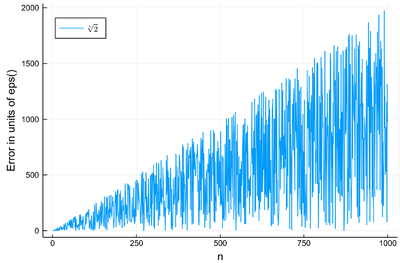
This is just to output, rather than to print, the value found, also grouping and compacting the above code:
julia> function bisection(f, a, b, maxit=100)
           c=(a+b)/2
           it=0
           while abs(f(c))>0 && it<maxit
               if f(a)*f(c)<0 b=c; else a=c; end
               c=(a+b)/2;
               it+=1;
           end
           abs(f(c)/eps())
       end
julia> plot(abs.(errbisec), label=L"\sqrt[n]{2}",
ylabel="Error in units of eps()", xlabel="n", legend=:topleft)
Expressing the form of the exact result is a problem for numerical analysis. The envelopes are fairly easy. Each oscillation is not noise but echoes the exact structure of floating points, and could be given explicitly. We find, in particular, that $\sqrt[1000]{2}\approx 1.000693387462[5807]$ with an error of 978$\times$eps() so we have put the last four digits in brackets but this is their 1000th power that departs from zero, so we could hope that they are actually also accurate. The exact result is in fact 1.00069338746258063 so only the last result is off as a result of rounding error and the result itself is optimal within machine precision.
We would feel that we have a great result, but if we remember the Babylonian method, this was much faster, doubling the number of accurate digits on each iteration while we merely increase by one digit of accuracy each time, so we are actually much worse! The Babylonian algorithm is indeed much more efficient in that instead of making a dichotomic improvement, it reduces the next interval accordingly to the magnitude of the function on its boundaries. Unknown to the Babylonians, this is actually implementing a particular case of the so-called Newton–Raphson method (Newton used it for the particular case of polynomials; Raphson extended it to arbitrary functions). The idea is to start with a blind guess $x_0$ around the solution and replace the real function $f(x)$ by a linear approximation with the same slope at $x_0$, i.e., $h(x)=f'(x_0)x+\beta$ with $\beta$ such that $h(x_0)=f(x_0)$ which yields
$$h(x)=f'(x_0)[x-x_0]+f(x_0)$$
Now a better guess for the zero is found by solving $h(x)=0$ which has solution $x=x_0-(f(x_0)/f'(x_0))$. Of course the procedure can be iterated so the algorithm gives us the always better approximations:
$$x_{n+1}=x_n-{f(x_n)\over f'(x_n)}\,.\label{eq:NewtRaph}$$
Babylonians meet Newton. Show that Eq. \eqref{eq:NewtRaph} applied to $f(x)=x^2-2$ yields the Babylonian formula $x_{n+1}={1\over2}\left(x_n+{2\over x_n}\right)$ to compute the square root of 2. Show that the corresponding formula for the cubic root of 2 is $$x_{n+1}={2\over 3}\left(x_n+{1\over x_n^2}\right)$$ and offer an expression for the general case. Check it numerically to the highest possible (machine) precision.
This is immediate since $f'(x)=2x$ and Newton--Raphson's method reads in this case \begin{equation} x_{n+1}=x_n-{f(x_n)\over f'(x_n)}=x_n-{x_n^2-2\over 2x_n}={x_n\over 2}+{1\over x_n}\,. \end{equation} Working out the general case first, i.e., with $f(x)=x^p-x_0$ for $\sqrt[p]{x_0}$ (that is generalizing both the power of the root and the value of the radicand), we find, since $f'(x)=px^{p-1}$: $$x_{n+1}=x_n(1-{1\over p})+{x_0\over px_n^{p-1}}$$ of which the result given is the particular case for $p=3$ and $x_0=2$. This checks it numerically (this computes $\sqrt[4]{5}$):
p=4;x0=5;
xn=x0;
xnp=xn+1;
it=0;
while abs(xnp-xn)>0 && it<25
    global xn=xnp;
    println("iteration $(it): $(global xnp=xn*(1-1/p)+x0/(p*xn^(p-1)))")
    global it+=1;
end

iteration 0: 4.505787037037037
iteration 1: 3.393004912578661
iteration 2: 2.57675416848638
iteration 3: 2.0056275413610223
iteration 4: 1.6591590888259025
iteration 5: 1.5180511192365604
iteration 6: 1.4958529904171414
iteration 7: 1.4953490360956547
iteration 8: 1.4953487812212858
iteration 9: 1.4953487812212205
iteration 10: 1.4953487812212205
This was for polynomials (actually, monomials), which is Newton's method. Let us go full Raphson-mode with a more complicated problem, e.g., let us find the zeros of $f(x)=\sin(x^2)$ between 0 and $\pi$. It's good to know beforehand the sort of results we expect (we added vertical lines by eye):
psin2=plot(x->sin(x^2), 0, π,
ylabel=L"\sin(x^2)",xlabel=L"x",lw=3,
legend=false)
vline!([0, 1.77, 2.51, 3.07], line = (:red, :dash, 1))
hline!([0], line = (:black, :dot, .75))
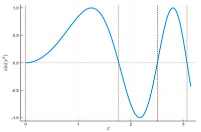
The formula gives us:
$$x_{n+1}=x_n-{\sin x_n^2\over 2x_n\cos x_n^2}$$
We can write a function that takes $f/f'$ as an input (that we have to compute ourselves) that computes such iterations until the procedure hits the best possible accuracy withing machine precision or overcome some number of iterations:
function NewtonRaphson(ffp, x0, maxint=50)
    it=0;
    x1=x0+1;
    while abs(x1-x0)>0 && it<maxint
        x0=x1
        x1=x0-ffp(x0)
    end
    x1
end
This provides the values found in the $[0,\pi]$ interval:
lsols=[NewtonRaphson(x->sin(x^2)/(2*x*cos(x^2)), x) for x in 0:.01:π]
We can plot the solutions together with where was the starting point:
psin2=plot(x->sin(x^2), 0, π,
label=L"\sin(x^2)",xlabel=L"x",
legend=:bottomleft)
scatter!((0:.01:pi, lsols), ylims=(-1,5), label="Zeros")
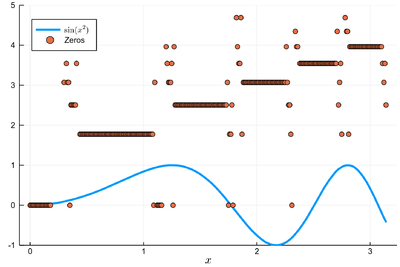
We found many, in particular some outside the $[0,\pi]$ range (this was the case when the tangent was sending us far away). We can check these are indeed all solutions:
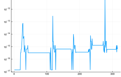
Interestingly, we found some subnormal solutions! This is a plotted version of the sought zeros, where we replace the numerical zero by a denormal number (appearing below the $10^{-16}$ horizontal on the plot):
plot(replace(abs.(sin.(lsols.^2)),0=>eps()/2^4), yscale=:log10, legend=false, lw=2)
To actually extract the values, we could use unique(), but this would return a lot of different values for the 0 zero, so we'd round this:
lsolss=sort(unique(round.(lsols,digits=10)))
These are the said solution in the sought range:
lsolss[findall(x-> 0<=x<=π, lsolss)]
5-element Array{Float64,1}:
 -0.0
  0.0
  1.7724538509
  2.5066282746
  3.0699801238
As we have transited through denormal numbers, we have the annoying but harmles occurrence of both -0.0 and 0.0. We have four solutions, as is clear from the initial graph.
One problem of the Newton-Raphson method is that it requires us to provide, and thus compute, the derivative of the function. In practice, we might not know it, not be willing to compute it or it might not even exist! Using the exact derivative provides the fastest convergence (the best guess) but it is not needed to be always spot on, it is often enough to provide a good-enough guess, namely, we could use the secant rather than the derivative, that is to say, the slope given by two points of the function, conveniently taken from the iterative procedure, rather than the exact tangent to the curve, which requires infinitesimals. Approximating $f'$ in Eq. \eqref{eq:NewtRaph}, we find:
$$x_{n+1}=x_n-f(x_n){x_n-x_{n-1}\over f(x_n)-f(x_{n-1})}={x_{n-1}f(x_n)-x_nf(x_{n-1})\over f(x_n)-f(x_{n-1})}$$
which, by the way, requires two starting points as opposed to the exact slope that is local. This is a possible julia implementation:
function secant(f, x0, x1, maxint=50)
    it=0;
    while abs(x1-x0)>0 && it<maxint
        println("$(x0)\t $(x1)");
        x2=x1
        x1=(x0*f(x1)-x1*f(x0))/(f(x1)-f(x0))
        x0=x2
        it+=1
    end
    x1
end
Now one can find the roots without assuming anything about the function, as was the case with our initial functions, in particular the bisection one, but much faster, and we can display the full output:
julia> secant(x->x^2-2,0,2)
0        2
2        1.0
1.0      1.3333333333333333
1.3333333333333333       1.4285714285714286
1.4285714285714286       1.4137931034482758
1.4137931034482758       1.41421143847487
1.41421143847487         1.4142135626888699
1.4142135626888699       1.414213562373095
1.414213562373095        1.4142135623730951
1.4142135623730951       1.414213562373095
1.414213562373095
It is only slightly less rapid than the exact Newton-Raphson version. Commenting the printing of the intermediate values, we can check that we recover the same zeros for the $\sin(x^2)$ functions (with the same precision):
julia> lsols=[secant(x->sin(x^2), x, x+1, 10) for x in 0:.01:π];
julia> lsolss[findall(x-> 0<=x<=π, lsolss)]
5-element Array{Float64,1}:
 -0.0
  0.0
  1.7724538509
  2.5066282746
  3.0699801238
but without having to differentiate ourselves any function. This is highly welcomed when the derivative, even if straightforward formally, turns out to be tedious to carry out.
Find all the zeros in $[0, 2\pi]$ of $f(x)=\sin(3x-x^2e^{-\sin(x)}/3)$.
The first thing is to have a broad idea of the solution we're looking for:
plot(x->sin(3x-x^2*exp(-sin(x))/3), 0,2pi,
     lw=3, xlabel="x", ylabel="f(x)", legend=false)
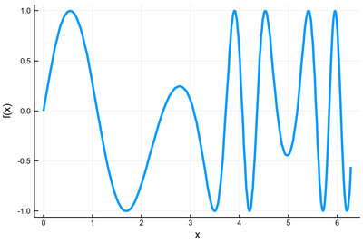
We are looking for the point where the curve intersects with the $x$-axis. So we are looking for 12 solutions. Here, on such a wildly varying function, it will be useful to upgrade our function to tackle potential problems of divisions by zeros:
function secant(f, x0, x1, maxint=50)
    it=0;
    while abs(x1-x0)>0 && it<maxint
#        println("$(x0)\t $(x1)");
        x2=x1
        Δf=f(x1)-f(x0)
        x1=(x0*f(x1)-x1*f(x0))/(Δf == 0 ? eps() : Δf)
        x0=x2
        it+=1
    end
    x1
end
Then, finding the initial points that make it work (find all the solutions), is an art mixing intuition and understanding of the method. After various attempts, some of them were missing the previous to last zero, we find that the following works:
lsols=[secant(x->sin(3x-x^2*exp(-sin(x))/3), x, x+1) for x∈0:.01:10]
lsolss=sort(unique(round.(lsols,digits=13)))
lsolsr=lsolss[findall(x-> 0<=x<=2π, lsolss)]
plot(x->sin(3x-x^2*exp(-sin(x))/3), 0, 2pi,
     lw=3, xlabel="x", ylabel="f(x)", legend=false)
scatter!((lsolsr, zeros(length(lsolsr))))
as is confirmed graphically:
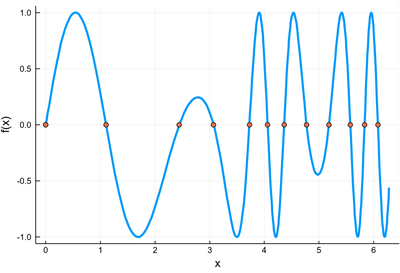
Zeros of $f(x)=\sin(3x-x^2e^{-\sin(x)}/3)$ superimposed on the function. Everything looks in order, we can trust the result.
Therefore with full confidence, we can take as solutions (we dropped the -0.0:
  0.0
  1.1025320443674
  2.4429256136412
  3.0711264580845
  3.726219257297
  4.0616487347151
  4.3623644077969
  4.7725103177739
  5.1833018782767
  5.5738924850625
  5.8349732442302
  6.0783486071141
There are many algorithms to find zeros of functions (you can consult Wikipedia's list). For instance, the so-called [1] aims at combining the exact Newton-Raphson method (using the derivative)'s speed of convergence with the secant's advantage of not requiring to know the derivative in the first place, by approximating it in another way. We let you study this (and other) root-finding algorithms. The ones we have provided should be enough to shed light on the big picture. And now that you know the basics, you can also rely more confidently on better or more robustly implemented routines. For instance, in julia, there is a Roots package that has a function fzero() that achieves something similar to what we've been trying to implement (the second parameter is the initial guess):
fzero(x->sin(x^2), 2)
1.772453850905516

fzero(x->sin(3x-x^2*exp(-sin(x))/3), 3)
3.071126458084516
You can read more about this function with ?fzero:
help?> fzero
search: fzero fzeros find_zero find_zeros find_zero! RoundFromZero finalizer UndefInitializer

  fzero(f, x0; order=0; kwargs...)
  fzero(f, x0, M; kwargs...)
  fzero(f, x0, M, N; kwargs...)
  fzero(f, x0; kwargs...)
  fzero(f, a::Number, b::Numbers; kwargs...)
  fzero(f, a::Number, b::Numbers; order=?, kwargs...)
  fzero(f, fp, a::Number; kwargs...)

  Find zero of a function using one of several iterative algorithms.

    •    f: a scalar function or callable object

    •    x0: an initial guess, a scalar value or tuple of two values

    •    order: An integer, symbol, or string indicating the algorithm to use for find_zero. The Order0 default may be specified directly by order=0, order=:0, or order="0"; Order1() by order=1, order=:1, order="1", or
        order=:secant; Order1B() by order="1B", etc.

    •    M: a specific method, as would be passed to find_zero, bypassing the use of the order keyword

    •    N: a specific bracketing method. When given, if a bracket is identified, method N will be used to finish instead of method M.

    •    a, b: When two values are passed along, if no order value is specified, Bisection will be used over the bracketing interval (a,b). If an order value is specified, the value of x0 will be set to (a,b) and the
        specified method will be used.

    •    fp: when fp is specified (assumed to compute the derivative of f), Newton's method will be used

    •    kwargs...: See find_zero for the specification of tolerances and other keyword arguments

  Examples:

  fzero(sin, 3)                  # use Order0() method, the default
  fzero(sin, 3, order=:secant)   # use secant method (also just `order=1`)
  fzero(sin, 3, Roots.Order1B()) # use secant method variant for multiple roots.
  fzero(sin, 3, 4)               # use bisection method over (3,4)
  fzero(sin, 3, 4, xatol=1e-6)   # use bisection method until |x_n - x_{n-1}| <= 1e-6
  fzero(sin, 3, 3.1, order=1)    # use secant method with x_0=3.0, x_1 = 3.1
  fzero(sin, (3, 3.1), order=2)  # use Steffensen's method with x_0=3.0, x_1 = 3.1
  fzero(sin, cos, 3)             # use Newton's method

  Note: unlike find_zero, fzero does not specialize on the type of the function argument. This has the advantage of making the first use of the function f faster, but subsequent uses slower.
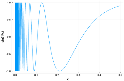
Zeros from hell: Find as many zeros as you can of the function $f(x)=\sin(1/x)$. We often use the computer as an easing way towards a solution that exact methods would not provide without considerable efforts. Sometimes, it is the other way around, since in this case the exact and full solution is fairly straightforward while a numerical one, which will always be almost fully incomplete, will turn into a nightmare. Confront yourself to hell and challenge your computer to this simple function. In case you'd like to use the exact Newton-Raphson method, we give you the easy part of the problem: $\sin(1/x)'=-\cos(1/x)/x^2$. Note that if we replace "hell" by "Float64", this impossible question only becomes a difficult one, with a unique solution.
