Crash Course in Scientific Computing
XVIII. Fitting
We have seen that interpolation works great theoretically but can lead to unpleasant results. Let alone Runge's phenomenon, we certainly do not want to constrain our model to pass by all points, taking into account irrelevant and meaningless fluctuations, noise, etc. While this is theoretically possible if we provide sufficient degrees of freedom, this is probably meaningless. What we typically want, instead, is the best overall agreement, without stretching too far our underlying model, which usually comes with its fixed number of degrees of freedom anyway. This problem is that of fitting, which is of extreme importance in most quantitative science.
Say that we have $N$ data points $y_1$, ..., $y_N$ obtained for the values $x_1$, ..., $x_N$ that we expect are accounted for by the "model" $f$, i.e., a function $f(x,\vec\beta)$ of $\nu$ parameters $\beta_1$, ..., $\beta_\nu$ kept in a vector $\vec\beta$:
$$r_i=f(x_i,\vec\beta)-y_i\,.$$
A good way to fit our data with the model is by minimizing the sum of the squared residuals (how much is left out by the model from the actual data):
$$S=\sum_{i=1}^N r_i^2\,.$$
We take the square as otherwise, positive and negative residuals would cancel without providing an exact fit. To find the optimum, that is, smallest, sum of squares, we vary $\beta$s such that $S$ is minimum, which is achieved when all $\partial S/\partial\beta_j$ terms for $1\le j\le\nu$ are canceled simultaneously:
$$\frac{\partial S}{\partial\beta_j}=2\sum_{i=1}^N(f(x_i,\vec\beta)-y_i)\frac{\partial f(x_i,\vec\beta)}{\partial\beta_j}=0\,,\quad\text{for $j=1,\dots,\nu$}\,.\label{eq:lstsq}$$
This is a complicated problem in general, that typically requires iterations over trials and errors.
There is a case where Eq. \ref{eq:lstsq} is considerably simplified, namely, if the partial derivative can be cancelled out, which occurs for so-called linear least squares where the parameters $\beta$ are merely linear coefficients of functions (that can be, of course, nonlinear). That is to say, our test function reads:
$$f(x;\vec\beta)=\sum_{k=1}^\nu\beta_k\phi_k(x)\,,$$
in which case:
$$\frac{\partial f(x_i;\beta)}{\partial\beta_j}=\phi_j(x_i)\,.$$
We put this back in each term of the differential in $\beta$:
$$\frac{\partial S}{\partial\beta_j}=2\sum_{i=1}^N\left(\left[\sum_{k=1}^\nu\beta_k\phi_k(x_i)\right]-y_i\right)\phi_j(x_i)=0$$
and now, it remains to rearrange this equality so that we can write it in matrix form. To do so, we have to remember these properties (and notations):
Concatenation:
$$\sum_k A_{ik}B_{kj}=(AB)_{ij}$$
Transposition:
$$A^T_{ij}=A_{ji}$$
so that our equation above becomes:
$$\sum_{i=1}^N\sum_{k=1}^\nu\beta_k\phi_k(x_i)\phi_j(x_i)=\sum_{i=1}^N y_i\phi_j(x_i)\,,$$
We introduce the matrix $\Phi$ such that:
$$\Phi_{ij}\equiv\phi_j(x_i)\label{eq:phi}\,,$$
in which case, with some further grouping and reassembling:
$$\sum_{k=1}^\nu\sum_{i=1}^N\Phi^T_{ji}\Phi_{ik}\beta_k=\sum_{i=1}^N \Phi_{ij}y_i\,,$$
So that we can get rid of the $i$ indices:
$$\sum_{k=1}^\nu(\Phi^T\Phi)_{jk}\beta_k=(\Phi^T\vec y)_j\,,$$
where $\vec y=(y_1,\dots,y_N)^T$, and now getting rid of $k$:
$$[(\Phi^T\Phi)\vec\beta]_j=(\Phi^T\vec y)_j\,,$$
with $\beta$ our vector of unknown parameters. As the equality holds for all $1\le j\le\nu$, it holds for the full vector, providing us with the final equation in its matrix form:
$$(\Phi^T\Phi)\vec\beta=\Phi^T\vec y\,.$$
Assuming $(\Phi^T\Phi)$ is well conditioned (in particular, not singular), we get the formal solution by brute force inversion:
$$\vec\beta=(\Phi^T\Phi)^{-1}\Phi^T\vec y\,.$$
The $(\Phi^T\Phi)^{-1}\Phi^T$ could be problematic if large (many fitting functions and/or many data points) and actually computed in this form, in which case one can see it as the notation for a so-called "pseudo-inverse" that deals with such an object in an efficient and stable way.
Let us now turn from the general theory to particular cases of interest.
By far, the most famous and used type of fitting is with a linear function, of the type:
$$f(x;\vec\beta)=\beta_0+x\beta_1\,.$$
This is known as linear regression. In this case, our matrix become simply:
$$\Phi^T\Phi=\pmatrix{ 1 & 1 & 1 & \dots\\ x_1 & x_2 & x_3 & \dots }\pmatrix{ 1 & x_1 \\ 1 & x_2 \\ 1 & x_3 \\ \vdots & \vdots } = \pmatrix{ N & \sum x_i\\ \sum x_i & \sum x_i^2 }\,,$$
The inverse of a $2\times2$ matrix is the inverse of its determinant times the matrix where diagonal elements are swapped and off-diagonal ones are changed sign, so:
$$(\Phi^T\Phi)^{-1} = \frac{1}{N\sum x_i^2-(\sum x_i)^2} \pmatrix{ \sum x_i^2 & -\sum x_i\\ -\sum x_i & N }\,, $$
and since:
$$\Phi^T y=\pmatrix{ \sum y_i \\ \sum x_iy_i }$$
this brings us to the final, so-called closed-form result:
$$\beta=(\Phi^T\Phi)^{-1}\Phi^T y= \frac{1}{N\sum x_i^2-(\sum x_i)^2} \pmatrix{ \sum x_i^2\sum y_i-\sum x_i\sum x_iy_i \\ -\sum x_i\sum y_i + N\sum x_iy_i& }\,, $$
which is also exact, but remains so even without the computer. These formulas are used by most people as coming from the theory black box. Now you know where this comes from.
This is a fairly academic example:
lx=1:10;
ly=[i+rand() for i=1:10]
10-element Array{Float64,1}:
  1.3463726018714324
  2.3056187528936714
  3.7587963568119616
  4.2059357874643535
  5.34037742719678
  6.128596673768494
  7.907569110885781
  8.313526388025155
  9.715937355885496
 10.248586978087038

denum=length(lx)*sum(lx.^2)-sum(lx)^2;
β1=(sum(lx.^2)*sum(ly)-sum(lx)*sum(lx.*ly))/denum
0.3718341106295129

β2=(-sum(lx)*sum(ly)+length(lx)*sum(lx.*ly))/denum
1.010054115029

scatter(lx, ly, xlabel="x", ylabel="y", legend=:topleft, label="data")
plot!(x->β1+β2*x, 0, 10, label="best linear fit")
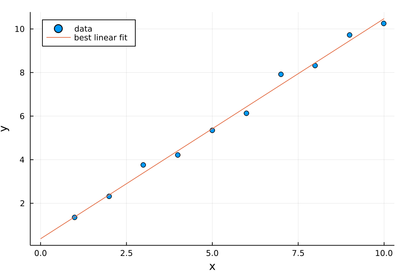
Note that from how we constructed the data, we expect $\beta_1=0.5$ and $\beta_2=1$ and the best fit values come out as approximately 0.37 and 1.01 respectively, with therefore a better guess at the slope than the intercept. We expect 0.5 from the intercept as we systematically add (never remove) the noise, thus causing a systematic error. It is not immediately clear why there is a better precision on the slope.
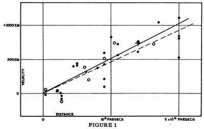
This data is from [1]:
| Distance (Mpc) | Radial velocity (km/sec) |
|---|---|
| 0.032 | 170 |
| 0.034 | 290 |
| 0.214 | -130 |
| 0.263 | -70 |
| 0.275 | -185 |
| 0.275 | -220 |
| 0.45 | 200 |
| 0.5 | 290 |
| 0.5 | 270 |
| 0.63 | 200 |
| 0.8 | 300 |
| 0.9 | -30 |
| 0.9 | 650 |
| 0.9 | 150 |
| 0.9 | 500 |
| 1.0 | 920 |
| 1.1 | 450 |
| 1.1 | 500 |
| 1.4 | 500 |
| 1.7 | 960 |
| 2.0 | 500 |
| 2.0 | 850 |
| 2.0 | 800 |
| 2.0 | 1090 |
A linear regression of this data (expand to access it) was one of the greatest results of astronomy, which led Einstein to lament that he had made the blunder of his life in introducing a cosmological constant, that made the observation, not the theory, predict the expansion of the universe. Find the Hubble's constant, which is the slope of these points. Note as well the unclear agreement between the data and the paper's figure.
Like we did for interpolation, let us now progress from the linear case to polynomials. For interpolation, we had the strong result that a polynomial of order $N-1$ could fit $N$ data points exactly. There is a stronger result for fitting with polynomials, known as the Weierstrass Approximation Theorem, which states that every continuous function defined on a closed interval can be uniformly approximated as closely as desired by a polynomial function. This shows again how fitting overcomes interpolation, which breaks down in the hand of Runge's phenomenon. Weierstrass shows, on the other hand, that polynomials are good enough to get arbitrarily close, as long as we do not demand them to be exact on particular values.
The result also follows from the general theory, in which case:
$$f(x;\beta)\equiv\sum_{k=0}^N\beta_k x^k$$
and our $\Phi$ matrix (which by the way goes by the name of a Gramian) reads:
$$\Phi=\pmatrix{ 1 & x_1 & x_1^2 & x_1^3 & \dots \\ 1 & x_2 & x_2^2 & x_2^3& \dots \\ \vdots & & & & \vdots \\ 1 & x_N & x_N^2 & x_N^3 & \dots }$$
Namely, for quadratic fitting, this reads:
$$\Phi=\pmatrix{ 1 & x_1 & x_1^2 \\ 1 & x_2 & x_2^2 \\ &\vdots & \\ 1 & x_N & x_N^2 } \quad\text{so that}\quad \vec\beta =(\Phi^\dagger\Phi)^{-1}\Phi^\dagger\vec y=\pmatrix{ N & \sum_{i=1}^N x_i & \sum_{i=1}^N x_i^2 \\ \sum_{i=1}^N x_i & \sum_{i=1}^N x_i^2 & \sum_{i=1}^N x_i^3 \\ \sum_{i=1}^N x_i^2 & \sum_{i=1}^N x_i^3 & \sum_{i=1}^N x_i^4 }^{-1}\pmatrix{\sum_{i=1}^N y_i \\ \sum_{i=1}^N y_i x_i \\ \sum_{i=1}^N y_i x_i^2} $$
which, being $3\times3$, can be inverted formally, to produce exact results. It is more convenient, however, to have the computation performed numerically. Let us turn to the computer, to best interpolate quadratically, say:
lx=[1, 2, 3, 5, 7];
ly=[3, 2, 2, 4, 11];
scatter(lx, ly, legend=false, xlabel="x", ylabel="y")
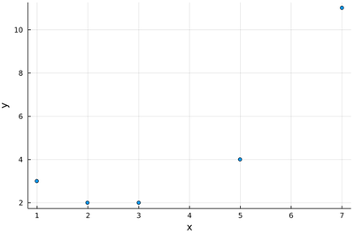
It looks reasonable that one will get a good quadratic fit to such data (and clearly not with a mere linear fit). We provide directly $\Phi^\dagger\Phi$:
ΦdΦ=[length(lx) sum(lx) sum(lx.^2);
            0 sum(lx.^2) sum(lx.^3);
            0 0 sum(lx.^4)]
ΦdΦ[2,1]=ΦdΦ[1,2];
ΦdΦ[3,1]=ΦdΦ[1,3];
ΦdΦ[3,2]=ΦdΦ[2,3];
we now have our matrix:
ΦdΦ
3×3 Array{Int64,2}:
  5   18    88
 18   88   504
 88  504  3124
and its numerical inverse:
inv(ΦdΦ)
3×3 Array{Float64,2}:
  2.78465   -1.58316    0.176972
 -1.58316    1.04957   -0.124733
  0.176972  -0.124733   0.0154584
and thus the best-fitting parameters:
beta=inv(ΦdΦ)*[sum(ly), sum(ly.*lx), sum(ly.*(lx.^2))]
3-element Array{Float64,1}:
  5.33262260127934
 -2.6982942430703787
  0.49893390191898135
which provide the best quadratic fit:
plot!(x->beta[1]+beta[2]*x+beta[3]*x^2, 0, 8)
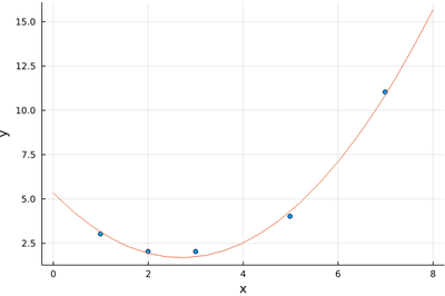
This is how close we manage to get:
(x->beta[1]+beta[2]*x+beta[3]*x^2).(lx)
5-element Array{Float64,1}:
  3.1332622601279425
  1.9317697228145079
  1.728144989339036
  4.31449893390198
 10.892324093816775
to the sought values:
ly
5-element Array{Int64,1}:
  3
  2
  2
  4
 11
with total squares of residuals:
sum(((x->beta[1]+beta[2]*x+beta[3]*x^2).(lx)-ly).^2)
0.2068230277185501
The statement is that no over parabola is such that the corresponding square distances get below this value. We have involved a numerical inverse. If we had recoursed to the exact result, we would have found the best parabola to be:
$$f(x)={2501\over469}-{2531\over938}x+{234\over469}x^2$$
with total squares of residuals $97/469$ which evaluates to the same numerical value that we have found above.
We now generalize the procedure to higher-order polynomials. This piece of code can do it for the general case, which we illustrate with n=3:
n=3
Φ=[0 for i in 1:length(lx), j in 1:n+1]

for i = 1:length(lx)
    for j = 1:n+1
        Φ[i,j]=lx[i]^(j-1)
    end
end

β=inv(transpose(Φ)*Φ)*(transpose(Φ)*ly)

plot!(x->sum(β[i]*x^(i-1) for i=1:n+1), 0,8, labels="order $(n)", legend=:topleft)
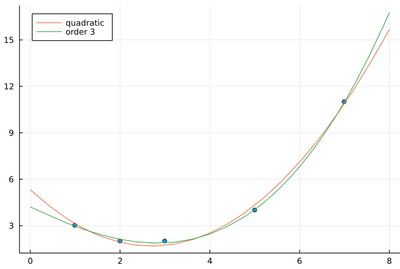
The sum of squared residuals is indeed now much smaller:
sum(((x->sum(β[i]*x^(i-1) for i=1:length(β))).(lx)-ly).^2)
0.03007518796992481
We have five data points. If we allow five degrees of freedom for our interpolating polynomial, namely, n=4, we get back to the interpolation case of passing through all the points:
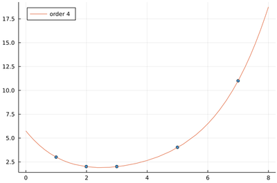
With the sum of squared residuals now (numerically) zero:
sum(((x->sum(β[i]*x^(i-1) for i=1:length(β))).(lx)-ly).^2)
2.8181138740886673e-19
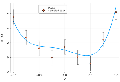
Define a polynomial "model" $m(x)$ of order $n$ (say $n=5$ with $-1\le x\le 1$), for instance by drawing coefficients randomly:
c=[rand(-10:10) for i=1:5]
function m(x)
    sum(c[i]x^(i-1) for i=1:length(c))
end
and simulate a measurement by randomly sampling $N$ points from this model with normally distributed noise around the theoretical value, e.g., this shows the result of such a sampling (equidistant on the $x$ axis) with a standard deviation set to $\sigma=1$:
lx=-1:.25:1;
plot(m, -1, 1, label="Model", legend=:topleft, lw=2, xlabel="x", ylabel="m(x)")
scatter!(lx, m.(lx)+randn(length(lx)), yerror=σ, label="Sampled data")
Find the best fit $f_k(x)$ with a polynomial of order $k$ for $0\le k\le n$ and compute
$$\chi^2\equiv\sum_{i=1}^N{(m(x)-f_k(x))^2\over\sigma^2}$$
Study the distribution of $\chi^2$ as a function of $k$. Such function (chi-square of degree $k$) are very important in the field of statistics for hypothesis testing.
We conclude with fitting with functions other than polynomials. In computer science, they typically provide enough generality, but in physics, many functional dependencies are of a different type. For instance, it is customary to encounter exponential behavior (which requires an infinite number of polynomials).
One can use the linear squares theory above as long as the coefficients $\beta$ weight a linear superposition of functions. Sometimes it could appear there is a clever trick to extend its reach. Say we have data distributed according to an exponential distribution (e.g., lifetimes of a radioactive sample of initial population $N(0)$ decaying at a rate $\gamma$):
$$N(t)=N(0)\exp(-\gamma t)$$
Then we could use the trick:
$$\ln(N(t))=\ln(N(0))-\gamma t$$
which is a linear function of the coefficients $(\ln N(0), \gamma$) and we could then use the analytical results above.
Tricks can be clever or they can be foolish and deceiving.
In this case, this is bad practice, since the noise is not distributed linearly, due to the nonlinear nature of the function. Therefore the regression analysis (the linear least square) biases the fit.
Let us simulate radioactive decay by sampling a thousand points according to the exponential distribution. We will need some packages to process the data:
using Random # for randexp()
using StatsBase # for fit()
An histogram can be computed (rather than plotted) through the fit function that returns an object:
myrandexp=fit(Histogram, randexp(1000), nbins=25)

Histogram{Int64,1,Tuple{StepRangeLen{Float64,Base.TwicePrecision{Float64},Base.TwicePrecision{Float64}}}}
edges:
  0.0:0.5:8.0
weights: [403, 239, 135, 75, 41, 38, 26, 17, 11, 4, 5, 4, 1, 0, 0, 1]
closed: left
isdensity: false
From this object, one can obtain the sought data as follows:
lt=collect(myrandexp.edges[1])
pop!(lt)
lNt=myrandexp.weights
with, in lt the $x$-axis values of the variable and in lNt the corresponding values of the data to fit. As we deal with logarithms, we will take care to remove possible zeros:
ix_zeroNt=findall(x->x==0, lNt)
deleteat!(lt, ix_zeroNt)
deleteat!(lNt, ix_zeroNt)
Now we can work with logarithms, which are linear on a log-scale, and can thus (presumably!) be fitted as a line:
logNt=log.(lNt)

denum=length(lt)*sum(lt.^2)-sum(lt)^2;
β1=(sum(lt.^2)*sum(logNt)-sum(lt)*sum(lt.*logNt))/denum
β2=(-sum(lt)*sum(logNt)+length(lt)*sum(lt.*logNt))/denum

scatter(lt, logNt, xlabel="t", ylabel="N(t)")
plot!(t->β1+β2*t, 0, maximum(lt)+.25, label="best linear fit of log-data")
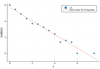
As a linear fit of a line, it is not a bad fit. It best passes through all the points. Which is precisely the problem: the small-value points have much more noise than the high-value ones, and thus should not be given that much weight. This becomes appreciable when going back to the linear scale, where the exponential is "exponential" again:
scatter(lt, lNt, xlabel="t", ylabel="N(t)")
plot!(t->exp(β1+β2*t), 0, maximum(lt)+.25, label="best exp fit of data by linear regression")
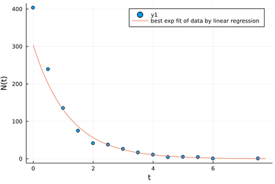
Clearly, seen as an exponential, this is not a good fit! It is very off for the most significant values, while it is optimum for the data linearized through the logarithms. This error comes from the rare long-time events, which have more noise, but that is taken as equally significant as the early time ones.
One should, instead, do a nonlinear fit. We do not present here algorithms to do so. The most famous one, if you are interested to further pursue the topic, is the Levenberg–Marquardt algorithm, that performs a gradient descent of nonlinear least squares. Here, we will turn to the black box magic instead and rely on someone's having implemented this algorithm for us. We can do so with the LsqFit package:
using LsqFit
m(t, p) = p[1] * exp.(p[2] * t)
p0 = [0.5, 0.5]
myfit = curve_fit(m, lt, lNt, p0)
LsqFit.LsqFitResult{Array{Float64,1},Array{Float64,1},Array{Float64,2},Array{Int64,1}}([402.63466262494325, -1.0661500557034478], [-0.3653373750567539, -2.7348766322302254, 3.639848233795192, 6.353554195006538, 6.738084428648058, -9.987398369171565, -9.562267746617358, -7.354375320265273, -5.339968918573802, -0.6787063662120771, -3.0510722921576914, -2.856373561266997, -0.3289225525881063, -0.8644067673380488], [0.9999999999970097 0.0; 0.5867977730190841 118.13256168246528; … ; 0.0016667155357003194 4.0264646854487305; 0.0003367649267284145 1.0169492453458406], true, Int64[])
This returns a LsqFitResult object, of which we can extract the following:
fit.dof: degrees of freedom
fit.param: best fit parameters
fit.resid: vector of residuals
fit.jacobian: estimated Jacobian at solution
so, in our case, as we want the parameters:
γ=myfit.param
2-element Array{Float64,1}:
 402.63466262494325
  -1.0661500557034478

plot!(t->γ[1]*exp(γ[2]*t), 0, maximum(lt)+.25, label="best exp fit by nonlinear fit")
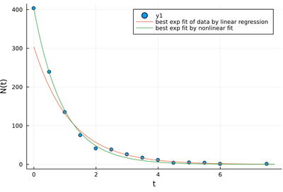
Fitting, being the process of matching a theoretical model to raw data, is one of the central operations in science in general and physics in particular. This lecture should have made clear, however, that the procedure itself is riddled with meaningless prowesses and deceiving pitfalls. This should explain Von Neumann's famous quote:
With four parameters I can fit an elephant, and with five I can make him wiggle his trunk.
.