Crash Course in Scientific Computing

XVIII. Differential calculus of vector fields

This page is still largely in progress.

We are now going to start looking at differential calculus in higher dimensions. Before we look at equations, in which case we tackle the general problem of partial differential equations, we consider derivatives of fields, either scalar or vector. A scalar can be regarded as a 1D vector so this lecture is about differential calculus of vector fields. We will focus on 2D fields for ease of visualisation but the principle would apply similarly to higher dimensions.

The main differential operators of vector calculus are:

1. gradient $\nabla f$
2. divergence $\nabla\cdot\vec F$
3. curl $\nabla\times\vec F$
4. Laplacian $\nabla^2 f$

for a scalar $f(x,y)$ and vector $\vec F(x,y)$ fields, respectively. The vectorf field consists itself of two scalar fields $F_x$ and $F_y$:

$$\vec F(x,y)\equiv F_x(x,y)\hat\imath+F_y(x,y)\hat\jmath$$

We can now remind the definitions and physical meaning of the differential operators (remember, in 2D):

1. $\nabla f=\begin{pmatrix}\partial_x f\\\partial_y f\end{pmatrix}$ measures the local rate of change of the function and thus points to the direction of steepest ascent (positive) or descent (negative).
2. $\nabla\cdot\vec F=\partial_x F_x+\partial_y F_y$ measures how much the field is locally "flowing", in or out depending on the sign, meaning that its value increase there or decreases.
3. $\nabla\times\vec F=(\partial_x F_y-\partial_y F_x)\hat k$ measures how much the field is locally circulating or rotating.
4. $\nabla^2 f=\partial_x^2 f+\partial_y^2f$ measures how much a field differs locally from its surroundings. Fields that are everywhere equal to the average of their surroundings are called "harmonic".

Derive the above results from a literal understanding of $\nabla$ as the vector $\begin{pmatrix}\partial_x\\\partial_y\end{pmatrix}$ and check the character of the resulting object in each case (scalar or vector).

The gradient is obtained from $\begin{pmatrix}u_1\\u_2\end{pmatrix}\alpha=\begin{pmatrix}u_1 \alpha\\u_2\alpha\end{pmatrix}$ where, however, we are careful not to commute $\alpha$ (here $f$) with the vectors components (which are, here, operators). It is, clearly, a vector, and provides both a direction (where the function is changing the most) and a magnitude (by how much it is changing).

The divergence is obtained by computing a scalar product $\vec u\cdot\vec v=u_xv_x+u_yv_y$ which gives the expression above. It is, as the name spells out, a scalar.

The vector product is specifically 3D (e.g., it does not apply to 4D objects) and is, in general and as the name again spells out, a vector. It can still still be defined for a 2D object, where it reduces to a vector in the third dimension (perpendicular to the field) as a consequence of its 3D origin. It can thus be considered, in this special case, as a scalar field as well: $\begin{vmatrix} \hat\imath & \hat\jmath & \hat k\\ \partial_x & \partial_y & 0\\ F_x & F_y & 0 \end{vmatrix} = \begin{pmatrix} 0\\0\\\partial_x F_y-\partial_y F_x \end{pmatrix}\,.$

The Laplacian can be seend as a dot product of nabla with itself, $\nabla^2=\nabla\cdot\nabla$, so that, following $\vec u^2=u_x^2+u_y^2$ we get the second-order differential expression given (where the "squaring" for operators means "apply twice").

... definition of grid ...

Starting with the gradient:

To fix idea, we will define a function that looks like a mountain landscape, as follows:

function f(x,y)
    (cos(x*y)*y*((x-0.5)^2+(y-0.15)))^2*exp(-x^2-y^2/2)
end

which, from Lecture 8, we can represent as a 3D landscape:

   wireframe(x,y,f, xlabel="x", ylabel="y", zlabel="Mountains", dpi=200)

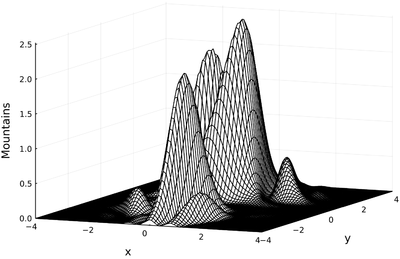
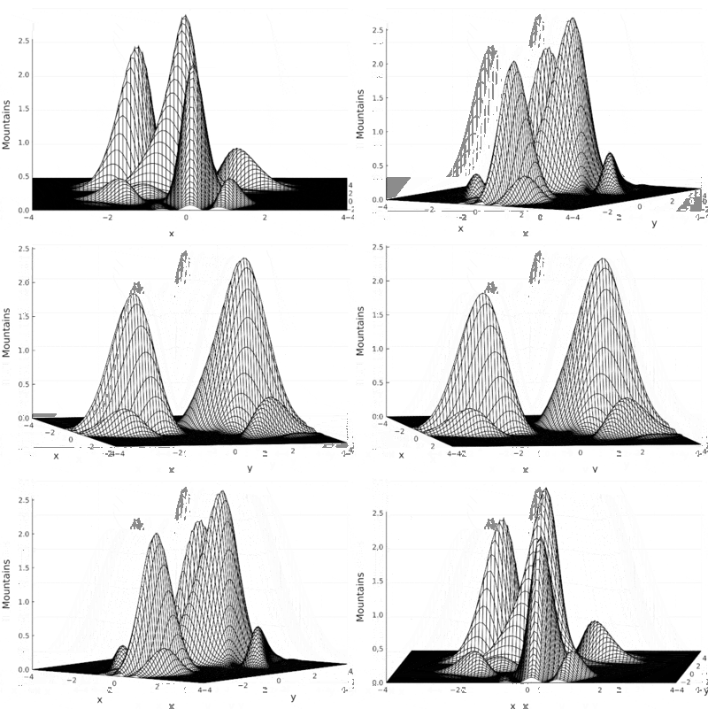
This is a 3D plot so it requires some mental flexibility to capture in its full complexity, in which case one can use an animation over the camera angle. There is a bug restricting the camera angle between 0 and 90°, so to make a seamless animation, we can loop back and forth using the vcat command:

julia> for i ∈ vcat(0:5:90, 85:-5:5)
           display(wireframe(x,y,f, xlabel="x", ylabel="y", zlabel="Mountains", camera=(i,20), dpi=200))
       #   print("$(i) ")
           sleep(0.1) 
       end

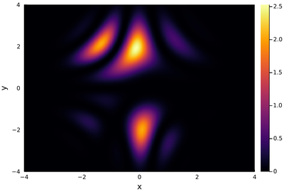
Beyond the 3D plot in relief and with perspective, we are often interested in a more accurate and quantitative picture, in which case we would use a density plot of our scalar field (sf), which we first discretize as this will be needed for our calculations anyway:

lx=-4:.01:4;
ly=-4:.01:4;
sf=[f(x,y) for y=lx, x=lx];

and then plot:

default(; xlabel="x", ylabel="y")
heatmap(lx, lx, sf)

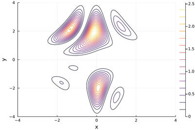
or only the isolines, which give us a familiar topographic feel of the scalar field:

contour(lx, lx, sf)

function Dx(myvec)
    (myvec[3]-myvec[1])/2
end

vfx=[Dx(sf[iy, ix-1:ix+1]) for iy ∈ 2:size(sf)[1]-1, ix ∈ 2:size(sf)[2]-1]

heatmap(slx, slx, ssf)
contour!(slx, slx, abs.(vfy), fill=false, lc=:white, lw=.1)

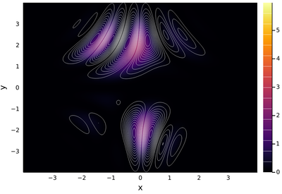
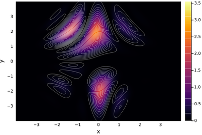
heatmap(slx, slx, ssf)
contour!(slx, slx, abs.(vfy), fill=false, lc=:white, lw=.1)

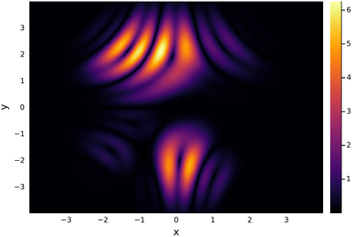
Modulus square:

heatmap(slx, slx, sqrt.(vfx.^2+vfy.^2))

The link between the discretized grid index $k$ and the continuous line $x$ is:

$$\begin{align} x&=k\delta x-4\\ k&={x+4\over\delta_x} \end{align}$$

so let us say we'd like to know the distanced climbed up from the center of the "map" to the mountain heading north. This is the profile, obtained as a vertical "cut" through the mountain landscape:

plot!(slx, ssf[:,400])

This is obtained as the sum over the little increases:

julia> sum(vfy[:,400][400:(round(Int,((2+4)/δx)))])*δx
2.3866293729048347

and should correspond to the elevation of the mountain at the final point (we started from 0):

julia> f(0,2)
2.3873143962938483

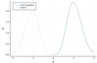
There is a numerical error, but the result is fairly accurate. We can in fact reconstruct it for any point of our journey:

plot(0:.01:3.9, [sum(vfy[:,400][400:ceil(Int,(x0+4)/δx)])*δx for x0=0:.01:3.9], xlabel="y", ylabel="h", label="From gradient")
plot!(slx, ssf[:,400], la=.25, lw=2, label="Exact", legend=:topleft)

We have headed north but the same would work vertically or along any line, in fact, along any trajectory:

Show numerically on the landscape provided that:

$$\int_{\vec a}^{\vec b}\nabla f\cdot d\vec r=f(\vec b)-f(\vec a)$$

We now turn to the divergence and curl, which apply to a vector field. In 2D, both return a scalar field, so they are pretty similar:

Now for the Laplacian, this one is interesting because it mixes the

We check that the following are harmonic functions:

we now turn to a different, matrix-form approach to the problem: