Elena & Fabrice's Web
This wikilog article is a draft, it was not published yet.
Crash course in Scientific Computing
m (→Crash Course in Scientific Computing) |
m (→Crash course in Julia (programming)) |
||
| (7 intermediate revisions by one user not shown) | |||
| Line 3: | Line 3: | ||
or, as officially known, [[The Wolverhampton Lectures on Physics]]: [[Wolverhampton Scientific Computing|VI — Scientific Computing]]. | or, as officially known, [[The Wolverhampton Lectures on Physics]]: [[Wolverhampton Scientific Computing|VI — Scientific Computing]]. | ||
| − | # [[ | + | {{WLPVI-content}} |
| − | # [[ | + | |
| − | # [[ | + | or do you mean |
| − | # [[WLV VI/ | + | |
| − | # [[WLV VI/ | + | # [[WLV VI/OS|Operating Systems]] |
| − | # [[WLV VI/VI|Random numbers]] | + | # [[WLV VI/TeX|$\TeX$ and $\LaTeX$]] |
| − | # [[WLV VI/ | + | # [[WLV VI/CP|Computer Programming]] |
| − | # [[WLV VI/ | + | # [[WLV VI/Julia|Julia]] |
| − | # [[WLV VI/ | + | # [[WLV VI/Plotting|Plotting]] |
| − | # [[WLV VI/ | + | # [[WLV VI/Numbers|Numbers]] |
| − | # [[WLV VI/ | + | # [[WLV VI/RandomNumbers|Random numbers]] |
| − | # [[WLV VI/ | + | # [[WLV VI/Algo1|Algorithms–the idea]] |
| − | # [[WLV VI/ | + | # [[WLV VI/Algo2|Algorithms–applications]] |
| − | # [[WLV VI/ | + | # [[WLV VI/Complexity|Complexity]] |
| − | # [[WLV VI/ | + | # [[WLV VI/Integrals|Integrals]] |
| − | # [[WLV VI/ | + | # [[WLV VI/Derivatives|Derivatives]] |
| − | # [[WLV VI/ | + | # [[WLV VI/Roots|Root finding]] |
| − | # [[WLV VI/ | + | # [[WLV VI/ODE1|ODE: Euler]] |
| − | # [[WLV VI/ | + | # [[WLV VI/ODE2|ODE: Heun & Runge-Kutta]] |
| − | # [[WLV VI/ | + | # [[WLV VI/ND|Higher Dimensions]] |
| − | # [[WLV VI/ | + | # [[WLV VI/LinearAlgebra|Linear algebra]] |
| − | # [[WLV VI/ | + | # [[WLV VI/DFT|Fourier and DFT]] |
| − | # [[WLV VI/ | + | # [[WLV VI/Interpolation|Interpolation]] |
| − | # [[WLV VI/ | + | # [[WLV VI/Extrapolation|Extrapolation]] |
| − | + | # [[WLV VI/Stability|Stability and Convergence]] | |
| + | # [[WLV VI/Chaos|Chaos and fractals]] | ||
| + | # [[WLV VI/OOP|Objects]] | ||
| + | # [[WLV VI/Lib|Librairies]] | ||
| + | # [[WLV VI/Fun|Fun problems]] | ||
| + | |||
| + | ---- | ||
| + | |||
| + | = Crash course in Julia (programming) = | ||
| + | |||
| + | When plotting pure functions, you might find that the density of points (PlotPoints in [[Mathematica]]) is not enough. This can be increased by specifying the step in the range, but in this case beware not to query your functions outside of its validity range, which would work otherwise. Compare: | ||
| + | |||
| + | <syntaxhighlight lang="python"> | ||
| + | plot(x->sqrt((15/x^2)-1),0,4,linewidth=5,linealpha=.5,linecolor=:red,ylims=(0,3)) | ||
| + | plot!(x->sqrt((15/x^2)-1),0:.0001:3.8729,linewidth=2,linecolor=:blue,ylims=(0,3)) | ||
| + | </syntaxhighlight> | ||
| + | |||
| + | <center><wz tip="High sampling-density (blue) vs automatic (red) but less trouble-making plot of a function that becomes ill-defined outside of its domain.">[[File:Screenshot_12-03-2020_184242.jpg|400px]]</wz></center> | ||
| + | |||
| + | The first version can plot over the range 0–4 but does so by not plotting the full function, while the second (with x-steps of 0.0001 allowing for the nice curvature) shows everything but would return an error if going over the limit where the argument gets negative. | ||
Latest revision as of 16:24, 8 March 2021
Crash Course in Scientific Computing
or, as officially known, The Wolverhampton Lectures on Physics: VI — Scientific Computing.
- Computers
- Operating Systems
- Software
- $\TeX$ and $\LaTeX$
- Computation
- Computer Programming
- Julia
- Plotting
- Numbers
- Random numbers
- Algorithms–the idea
- Algorithms–applications
- Root finding
- Linear Equations
- Interpolation and Extrapolation
- Fitting
- Integrals
- Derivatives
- Ordinary Differential Equations
- Differential calculus of vector fields
- Partial Differential Equations
- Finite elements and finite volumes
- Fourier and DFT
- Chaos and fractals
- Fun problems
or do you mean
- Operating Systems
- $\TeX$ and $\LaTeX$
- Computer Programming
- Julia
- Plotting
- Numbers
- Random numbers
- Algorithms–the idea
- Algorithms–applications
- Complexity
- Integrals
- Derivatives
- Root finding
- ODE: Euler
- ODE: Heun & Runge-Kutta
- Higher Dimensions
- Linear algebra
- Fourier and DFT
- Interpolation
- Extrapolation
- Stability and Convergence
- Chaos and fractals
- Objects
- Librairies
- Fun problems
Crash course in Julia (programming)
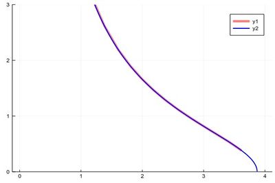
When plotting pure functions, you might find that the density of points (PlotPoints in Mathematica) is not enough. This can be increased by specifying the step in the range, but in this case beware not to query your functions outside of its validity range, which would work otherwise. Compare:
plot(x->sqrt((15/x^2)-1),0,4,linewidth=5,linealpha=.5,linecolor=:red,ylims=(0,3))
plot!(x->sqrt((15/x^2)-1),0:.0001:3.8729,linewidth=2,linecolor=:blue,ylims=(0,3))

The first version can plot over the range 0–4 but does so by not plotting the full function, while the second (with x-steps of 0.0001 allowing for the nice curvature) shows everything but would return an error if going over the limit where the argument gets negative.