m (Fabrice moved page WLV VI/ODE2 to WLP VI/ODE2) |
m |
||
| Line 1: | Line 1: | ||
| − | We | + | = Crash Course in Scientific Computing = |
| + | == XVIII. Runge-Kutta == | ||
| + | |||
| + | We now cover one of the most powerful predictor-corrector algorithms of all, | ||
| + | one which is so accurate that most computer algorithms use it as default: the fourth-order Runge-Kutta Method. RK methods are optimized predictor-corrector methods, so they push the idea of Heun's method to the top. The RK4 method finds the optimum correction-prediction (in a way which we do not detail here) to involve these intermediate points: | ||
| + | |||
| + | \begin{align} | ||
| + | k_1 &= h\ f(t_n, y_n)\,, \\ | ||
| + | k_2 &= h\ f\left(t_n + \frac{h}{2}, y_n + \frac{k_1}{2}\right)\,, \\ | ||
| + | k_3 &= h\ f\left(t_n + \frac{h}{2}, y_n + \frac{k_2}{2}\right)\,, \\ | ||
| + | k_4 &= h\ f\left(t_n + h, y_n + k_3\right)\,, | ||
| + | \end{align} | ||
| + | |||
| + | and then the calculation is explicit: | ||
| + | |||
| + | \begin{align} | ||
| + | t_{n+1} &= t_n + h\,, \\ | ||
| + | y_{n+1} &= y_n + \tfrac{1}{6}\left(k_1 + 2k_2 + 2k_3 + k_4 \right)\,. | ||
| + | \end{align} | ||
| + | |||
| + | In code: | ||
| + | <syntaxhighlight lang="python"> | ||
| + | @time for n=1:npts-1 | ||
| + | tn=(n-1)*h-t0; | ||
| + | k1=h*f(tn,y[n]); | ||
| + | k2=h*f(tn+(h/2),y[n]+k1/2); | ||
| + | k3=h*f(tn+(h/2),y[n]+k2/2); | ||
| + | k4=h*f(tn+h,y[n]+k3); | ||
| + | y[n+1]=y[n]+(1/6)*(k1+2*k2+2*k3+k4) | ||
| + | end | ||
| + | </syntaxhighlight> | ||
| + | |||
| + | The error analysis on the same problems as above now yields a very different result: | ||
| + | |||
| + | <syntaxhighlight lang="python"> | ||
| + | herror=[]; | ||
| + | for h in hlist | ||
| + | npts=round(Int64,tmax/h); | ||
| + | y=0.0*collect(1:npts); | ||
| + | y[1]=-24/37; | ||
| + | @time for n=1:npts-1 | ||
| + | tn=(n-1)*h; | ||
| + | k1=h*f(tn,y[n]); | ||
| + | k2=h*f(tn+(h/2),y[n]+k1/2); | ||
| + | k3=h*f(tn+(h/2),y[n]+k2/2); | ||
| + | k4=h*f(tn+h,y[n]+k3); | ||
| + | y[n+1]=y[n]+(1/6)*(k1+2*k2+2*k3+k4) | ||
| + | end | ||
| + | append!(herror,mean(abs.([-(24/37)*cos(3t)-(4/37)*sin(3t) for t in ((1:npts).-1).*h]-y))) | ||
| + | end | ||
| + | </syntaxhighlight> | ||
| + | |||
| + | <pre> | ||
| + | 0.006093 seconds (3.91 k allocations: 64.688 KiB) | ||
| + | 0.007069 seconds (41.92 k allocations: 674.766 KiB) | ||
| + | 0.071775 seconds (437.74 k allocations: 6.871 MiB) | ||
| + | 0.805397 seconds (4.40 M allocations: 68.998 MiB, 1.76% gc time) | ||
| + | 6.734973 seconds (43.98 M allocations: 690.260 MiB, 1.41% gc time) | ||
| + | 77.495034 seconds (439.82 M allocations: 6.741 GiB, 1.57% gc time) | ||
| + | </pre> | ||
| + | |||
| + | <syntaxhighlight lang="python"> | ||
| + | scatter(herror, xlabel="time step", ylabel="mean abs error", | ||
| + | xticks=(1:6, string.(hlist)), legend=false, yscale=:log10) | ||
| + | plot!(x->10^4*herror[1]*10.0^-(4x), 1, 6, ls=:dot, lw=3, ylims=(10^-15,10^-3)) | ||
| + | </syntaxhighlight> | ||
| + | |||
| + | <center><wz tip="Fourth-order accuracy of the RK4 method, which is so good that it quickly overtakes machine precision.">[[File:Screenshot_17-03-2020_114210.jpg|400px]]</wz></center> | ||
| + | |||
| + | The gain from $h=0.001$ to $h=0.0001$ is marginally better, and for smaller still $h$, it actually becomes worse, due to rounding errors. It works so well that many, if not most, resources would use the RK4 to integrate ODE. | ||
| + | |||
| + | We now turn to the case of coupled equations, in which case the method reads | ||
| + | |||
| + | $$\vec y'=\vec f(t,\vec y)$$ | ||
| + | |||
| + | where | ||
| + | |||
| + | $$ | ||
| + | \vec y\equiv | ||
| + | \begin{pmatrix} | ||
| + | y_1\\y_2 | ||
| + | \end{pmatrix} | ||
| + | \quad\text{and}\quad | ||
| + | \vec f\equiv | ||
| + | \begin{pmatrix} | ||
| + | f_1\\f_2 | ||
| + | \end{pmatrix}\,. | ||
| + | $$ | ||
| + | |||
| + | The methods are the same as before just applying directly to the vectors instead. An interesting ''coupled'' system of ODE, namely, the [https://en.wikipedia.org/wiki/Lotka%E2%80%93Volterra_equations Volterra-Lotka model of prey-predator] interactions. This is modelled with the pair of coupled ODE: | ||
| + | |||
| + | \begin{align} | ||
| + | \frac{dx}{dt} &= \alpha x - \beta x y, \\ | ||
| + | \frac{dy}{dt} &= \delta x y - \gamma y, | ||
| + | \end{align} | ||
| + | |||
| + | The functions are implemented as: | ||
| + | |||
| + | <syntaxhighlight lang="python"> | ||
| + | function f1(t,y1, y2) | ||
| + | α*y1-β*y1*y2 | ||
| + | end | ||
| + | function f2(t,y1, y2) | ||
| + | δ*y1*y2-γ*y2 | ||
| + | end | ||
| + | </syntaxhighlight> | ||
| + | |||
| + | Some common initialization for all methods, in particular, we now need two arrays of values to store the evolution of $x$ (in <tt>y1</tt>) and $y$ (in <tt>y2</tt>): | ||
| + | |||
| + | <syntaxhighlight lang="python"> | ||
| + | tmax=100 | ||
| + | h=.001 | ||
| + | npts=round(Int,tmax/h) | ||
| + | |||
| + | y1=0.0*collect(1:npts); | ||
| + | y2=0.0*collect(1:npts); | ||
| + | |||
| + | y1[1]=1; | ||
| + | y2[1]=.1; | ||
| + | |||
| + | α=2/3; | ||
| + | β=4/3; | ||
| + | γ=1; | ||
| + | δ=1; | ||
| + | </syntaxhighlight> | ||
| + | |||
| + | Euler's method in this case reads: | ||
| + | |||
| + | $$\vec y_{n+1}=\vec y_n+h\vec f(t_n,\vec y_n)$$ | ||
| + | |||
| + | or, breaking down this equation componentwise: | ||
| + | |||
| + | $$\begin{align} | ||
| + | y_{1,n+1}&=y_{1,n}+hf_1(t_n,y_{1,n},y_{2,n})\\ | ||
| + | y_{2,n+1}&=y_{2,n}+hf_2(t_n,y_{1,n},y_{2,n}) | ||
| + | \end{align}$$ | ||
| + | |||
| + | In code: | ||
| + | <syntaxhighlight lang="python"> | ||
| + | @time for i=1:npts-1 | ||
| + | y1[i+1]=y1[i]+h*f1((i-1)*h,y1[i],y2[i]) | ||
| + | y2[i+1]=y2[i]+h*f2((i-1)*h,y1[i],y2[i]) | ||
| + | end | ||
| + | </syntaxhighlight> | ||
| + | |||
| + | Heun's version reads: | ||
| + | |||
| + | $$\vec y_{n+1}=\vec y_n+{h\over 2}\left(\vec f(t_n,\vec y_n)+\vec f(t_{n+1},\vec y_n+h\vec f(t_i,\vec y_n)\right)$$ | ||
| + | |||
| + | or, breaking down this equation componentwise: | ||
| + | |||
| + | $$\begin{align} | ||
| + | y_{1,n+1} &= y_{1,n} + {h\over2} [f(t_n, y_{1,n}, y_{2,n}) + f(t_n + h, y_{1,n} + h f(t_n, y_{1,n}, y_{2,n}), y_{2,n})]\\ | ||
| + | y_{2,n+1} &= y_{2,n} + {h\over2} [f(t_n, y_{1,n}, y_{2,n}) + f(t_n + h, y_{1,n}, y_{2,n} + h f(t_n, y_{1,n}, y_{2,n}))] | ||
| + | \end{align}$$ | ||
| + | |||
| + | In code; where this time we'll find both more convenient and efficient to define auxiliary quantities, that are furthermore invoked more than once: | ||
| + | |||
| + | <syntaxhighlight lang="python"> | ||
| + | @time for n=1:npts-1 | ||
| + | tn=(n-1)*h; | ||
| + | f1left=f1(tn,yH1[n],yH2[n]) | ||
| + | f2left=f2(tn,yH1[n],yH2[n]) | ||
| + | f1right=f1(tn+h,yH1[n]+h*f1left,yH2[n]+h*f2left) | ||
| + | f2right=f2(tn+h,yH1[n]+h*f1left,yH2[n]+h*f2left) | ||
| + | yH1[n+1]=yH1[n]+(h/2)*(f1left+f1right) | ||
| + | yH2[n+1]=yH2[n]+(h/2)*(f2left+f2right) | ||
| + | end | ||
| + | </syntaxhighlight> | ||
| + | |||
| + | RK4's version reads: | ||
| + | |||
| + | $$ | ||
| + | \begin{align} | ||
| + | t_{n+1} &= t_n + h\,, \\ | ||
| + | \vec y_{n+1} &= \vec y_n + \tfrac{1}{6}\left(\vec k_1 + 2\vec k_2 + 2\vec k_3 + \vec k_4 \right)\,. | ||
| + | \end{align} | ||
| + | $$ | ||
| + | |||
| + | in terms of the intermediate quantities: | ||
| + | |||
| + | $$ | ||
| + | \begin{align} | ||
| + | \vec k_1 &= h\vec f(t_n, \vec y_n)\,, \\ | ||
| + | \vec k_2 &= h\vec f\left(t_n + \frac{h}{2}, \vec y_n + \frac{\vec k_1}{2}\right)\,, \\ | ||
| + | \vec k_3 &= h\vec f\left(t_n + \frac{h}{2}, \vec y_n + \frac{\vec k_2}{2}\right)\,, \\ | ||
| + | \vec k_4 &= h\vec f\left(t_n + h, \vec y_n + \vec k_3\right)\,, | ||
| + | \end{align} | ||
| + | $$ | ||
| + | |||
| + | In code | ||
| + | <syntaxhighlight lang="python"> | ||
| + | @time for n=1:npts-1 | ||
| + | tn=(n-1)*h; | ||
| + | # Intermediate steps | ||
| + | k11=h*f1(tn,yRK1[n],yRK2[n]); | ||
| + | k12=h*f2(tn,yRK1[n],yRK2[n]); | ||
| + | k21=h*f1(tn+(h/2),yRK1[n]+k11/2,yRK2[n]+k12/2); | ||
| + | k22=h*f2(tn+(h/2),yRK1[n]+k11/2,yRK2[n]+k12/2); | ||
| + | k31=h*f1(tn+(h/2),yRK1[n]+k21/2,yRK2[n]+k22/2); | ||
| + | k32=h*f2(tn+(h/2),yRK1[n]+k21/2,yRK2[n]+k22/2); | ||
| + | k41=h*f1(tn+h,yRK1[n]+k31,yRK2[n]+k32); | ||
| + | k42=h*f2(tn+h,yRK1[n]+k31,yRK2[n]+k32); | ||
| + | # Real step | ||
| + | yRK1[n+1]=yRK1[n]+(1/6)*(k11+2*k21+2*k31+k41); | ||
| + | yRK2[n+1]=yRK2[n]+(1/6)*(k12+2*k22+2*k32+k42); | ||
| + | end | ||
| + | </syntaxhighlight> | ||
| + | |||
| + | Results can be shown in two ways: | ||
| + | |||
| + | 1 - As the respective solutions. This shows the oscillations of predators and preys | ||
| + | |||
| + | <syntaxhighlight lang="python"> | ||
| + | pRK=plot([[yRK1[i] for i=1:240], [yRK2[i] for i=1:240]], | ||
| + | lw=3, xlabel="time", ylabel="populations", label="RK4") | ||
| + | </syntaxhighlight> | ||
| + | |||
| + | <center><wz tip="Predators & Preys dynamics according to Volterra-Lotka equations, here simulated with the RK4 method.">[[File:Screenshot_18-03-2020_104336.jpg|400px]]</wz></center> | ||
| + | |||
| + | 2 - As a phase-space solution, showing the simultaneous state of the system (here, ecosystem), with time as a parametric parameter: | ||
| + | |||
| + | <syntaxhighlight lang="python"> | ||
| + | psRK=plot([(yRK1[i], yRK2[i]) for i=1:npts], | ||
| + | lw=1, xlabel="x", ylabel="y", legend=false) | ||
| + | </syntaxhighlight> | ||
| + | |||
| + | <center><wz tip="Phase-space solution of the Volterra-Lotka equations, still with RK4, over about 70 cycles.">[[File:Screenshot_18-03-2020_112201.jpg|400px]]</wz></center> | ||
| + | |||
| + | This comparing the three methods together (the various plots have been evaluated as <tt>pE</tt>, <tt>pH</tt>, etc.): | ||
| + | |||
| + | <syntaxhighlight lang="python"> | ||
| + | plot(pE,pH,pRK,psE,psH,psRK,layout=(2,3),dpi=150) | ||
| + | </syntaxhighlight> | ||
| + | |||
| + | <center><wz tip="Volterra-Lotka as simulated by Euler (quickly diverges), Heun (good but a small drift) & RK4 (perfect).">[[File:Screenshot_18-03-2020_103544.jpg|650px]]</wz></center> | ||
| + | |||
| + | The time-evolutions at the top are over considerably fewer cycles for Heun & RK4 methods than those simulated to produce the phase space solutions, bottom. You can see how the RK4 method stays stable (which is the correct behaviour) while the Heun method slowly drifts towards the stable point. | ||
{{WLP6}} | {{WLP6}} | ||
Revision as of 16:25, 8 March 2021
Crash Course in Scientific Computing
XVIII. Runge-Kutta
We now cover one of the most powerful predictor-corrector algorithms of all, one which is so accurate that most computer algorithms use it as default: the fourth-order Runge-Kutta Method. RK methods are optimized predictor-corrector methods, so they push the idea of Heun's method to the top. The RK4 method finds the optimum correction-prediction (in a way which we do not detail here) to involve these intermediate points:
\begin{align} k_1 &= h\ f(t_n, y_n)\,, \\ k_2 &= h\ f\left(t_n + \frac{h}{2}, y_n + \frac{k_1}{2}\right)\,, \\ k_3 &= h\ f\left(t_n + \frac{h}{2}, y_n + \frac{k_2}{2}\right)\,, \\ k_4 &= h\ f\left(t_n + h, y_n + k_3\right)\,, \end{align}
and then the calculation is explicit:
\begin{align} t_{n+1} &= t_n + h\,, \\ y_{n+1} &= y_n + \tfrac{1}{6}\left(k_1 + 2k_2 + 2k_3 + k_4 \right)\,. \end{align}
In code:
@time for n=1:npts-1
    tn=(n-1)*h-t0;
    k1=h*f(tn,y[n]);
    k2=h*f(tn+(h/2),y[n]+k1/2);
    k3=h*f(tn+(h/2),y[n]+k2/2);
    k4=h*f(tn+h,y[n]+k3);
    y[n+1]=y[n]+(1/6)*(k1+2*k2+2*k3+k4)
end
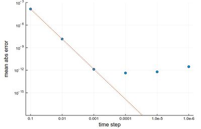
The error analysis on the same problems as above now yields a very different result:
herror=[];
for h in hlist
    npts=round(Int64,tmax/h);
    y=0.0*collect(1:npts);
    y[1]=-24/37;
    @time for n=1:npts-1
        tn=(n-1)*h;
        k1=h*f(tn,y[n]);
        k2=h*f(tn+(h/2),y[n]+k1/2);
        k3=h*f(tn+(h/2),y[n]+k2/2);
        k4=h*f(tn+h,y[n]+k3);
        y[n+1]=y[n]+(1/6)*(k1+2*k2+2*k3+k4)
    end
    append!(herror,mean(abs.([-(24/37)*cos(3t)-(4/37)*sin(3t) for t in ((1:npts).-1).*h]-y)))
end
  0.006093 seconds (3.91 k allocations: 64.688 KiB)
  0.007069 seconds (41.92 k allocations: 674.766 KiB)
  0.071775 seconds (437.74 k allocations: 6.871 MiB)
  0.805397 seconds (4.40 M allocations: 68.998 MiB, 1.76% gc time)
  6.734973 seconds (43.98 M allocations: 690.260 MiB, 1.41% gc time)
 77.495034 seconds (439.82 M allocations: 6.741 GiB, 1.57% gc time)
scatter(herror, xlabel="time step", ylabel="mean abs error",
    xticks=(1:6, string.(hlist)), legend=false, yscale=:log10)
plot!(x->10^4*herror[1]*10.0^-(4x), 1, 6, ls=:dot, lw=3, ylims=(10^-15,10^-3))

The gain from $h=0.001$ to $h=0.0001$ is marginally better, and for smaller still $h$, it actually becomes worse, due to rounding errors. It works so well that many, if not most, resources would use the RK4 to integrate ODE.
We now turn to the case of coupled equations, in which case the method reads
$$\vec y'=\vec f(t,\vec y)$$
where
$$ \vec y\equiv \begin{pmatrix} y_1\\y_2 \end{pmatrix} \quad\text{and}\quad \vec f\equiv \begin{pmatrix} f_1\\f_2 \end{pmatrix}\,. $$
The methods are the same as before just applying directly to the vectors instead. An interesting coupled system of ODE, namely, the Volterra-Lotka model of prey-predator interactions. This is modelled with the pair of coupled ODE:
\begin{align} \frac{dx}{dt} &= \alpha x - \beta x y, \\ \frac{dy}{dt} &= \delta x y - \gamma y, \end{align}
The functions are implemented as:
function f1(t,y1, y2)
    α*y1-β*y1*y2
end
function f2(t,y1, y2)
    δ*y1*y2-γ*y2
end
Some common initialization for all methods, in particular, we now need two arrays of values to store the evolution of $x$ (in y1) and $y$ (in y2):
tmax=100
h=.001
npts=round(Int,tmax/h)

y1=0.0*collect(1:npts);
y2=0.0*collect(1:npts);

y1[1]=1;
y2[1]=.1;

α=2/3;
β=4/3;
γ=1;
δ=1;
Euler's method in this case reads:
$$\vec y_{n+1}=\vec y_n+h\vec f(t_n,\vec y_n)$$
or, breaking down this equation componentwise:
$$\begin{align} y_{1,n+1}&=y_{1,n}+hf_1(t_n,y_{1,n},y_{2,n})\\ y_{2,n+1}&=y_{2,n}+hf_2(t_n,y_{1,n},y_{2,n}) \end{align}$$
In code:
@time for i=1:npts-1
    y1[i+1]=y1[i]+h*f1((i-1)*h,y1[i],y2[i])
    y2[i+1]=y2[i]+h*f2((i-1)*h,y1[i],y2[i])
end
Heun's version reads:
$$\vec y_{n+1}=\vec y_n+{h\over 2}\left(\vec f(t_n,\vec y_n)+\vec f(t_{n+1},\vec y_n+h\vec f(t_i,\vec y_n)\right)$$
or, breaking down this equation componentwise:
$$\begin{align} y_{1,n+1} &= y_{1,n} + {h\over2} [f(t_n, y_{1,n}, y_{2,n}) + f(t_n + h, y_{1,n} + h f(t_n, y_{1,n}, y_{2,n}), y_{2,n})]\\ y_{2,n+1} &= y_{2,n} + {h\over2} [f(t_n, y_{1,n}, y_{2,n}) + f(t_n + h, y_{1,n}, y_{2,n} + h f(t_n, y_{1,n}, y_{2,n}))] \end{align}$$
In code; where this time we'll find both more convenient and efficient to define auxiliary quantities, that are furthermore invoked more than once:
@time for n=1:npts-1
    tn=(n-1)*h;
    f1left=f1(tn,yH1[n],yH2[n])
    f2left=f2(tn,yH1[n],yH2[n])
    f1right=f1(tn+h,yH1[n]+h*f1left,yH2[n]+h*f2left)
    f2right=f2(tn+h,yH1[n]+h*f1left,yH2[n]+h*f2left)
    yH1[n+1]=yH1[n]+(h/2)*(f1left+f1right)
    yH2[n+1]=yH2[n]+(h/2)*(f2left+f2right)
end
RK4's version reads:
$$ \begin{align} t_{n+1} &= t_n + h\,, \\ \vec y_{n+1} &= \vec y_n + \tfrac{1}{6}\left(\vec k_1 + 2\vec k_2 + 2\vec k_3 + \vec k_4 \right)\,. \end{align} $$
in terms of the intermediate quantities:
$$ \begin{align} \vec k_1 &= h\vec f(t_n, \vec y_n)\,, \\ \vec k_2 &= h\vec f\left(t_n + \frac{h}{2}, \vec y_n + \frac{\vec k_1}{2}\right)\,, \\ \vec k_3 &= h\vec f\left(t_n + \frac{h}{2}, \vec y_n + \frac{\vec k_2}{2}\right)\,, \\ \vec k_4 &= h\vec f\left(t_n + h, \vec y_n + \vec k_3\right)\,, \end{align} $$
In code
@time for n=1:npts-1
    tn=(n-1)*h;
    # Intermediate steps
    k11=h*f1(tn,yRK1[n],yRK2[n]);
    k12=h*f2(tn,yRK1[n],yRK2[n]);
    k21=h*f1(tn+(h/2),yRK1[n]+k11/2,yRK2[n]+k12/2);
    k22=h*f2(tn+(h/2),yRK1[n]+k11/2,yRK2[n]+k12/2);
    k31=h*f1(tn+(h/2),yRK1[n]+k21/2,yRK2[n]+k22/2);
    k32=h*f2(tn+(h/2),yRK1[n]+k21/2,yRK2[n]+k22/2);
    k41=h*f1(tn+h,yRK1[n]+k31,yRK2[n]+k32);
    k42=h*f2(tn+h,yRK1[n]+k31,yRK2[n]+k32);
    # Real step
    yRK1[n+1]=yRK1[n]+(1/6)*(k11+2*k21+2*k31+k41);
    yRK2[n+1]=yRK2[n]+(1/6)*(k12+2*k22+2*k32+k42);
end
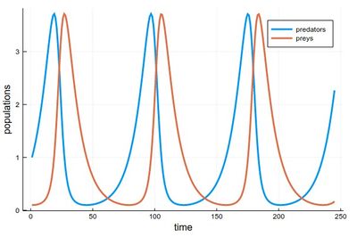
Results can be shown in two ways:
1 - As the respective solutions. This shows the oscillations of predators and preys
pRK=plot([[yRK1[i] for i=1:240], [yRK2[i] for i=1:240]],
lw=3, xlabel="time", ylabel="populations", label="RK4")

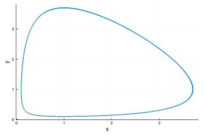
2 - As a phase-space solution, showing the simultaneous state of the system (here, ecosystem), with time as a parametric parameter:
psRK=plot([(yRK1[i], yRK2[i]) for i=1:npts],
lw=1, xlabel="x", ylabel="y", legend=false)

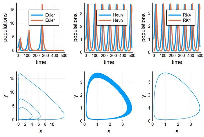
This comparing the three methods together (the various plots have been evaluated as pE, pH, etc.):
plot(pE,pH,pRK,psE,psH,psRK,layout=(2,3),dpi=150)

The time-evolutions at the top are over considerably fewer cycles for Heun & RK4 methods than those simulated to produce the phase space solutions, bottom. You can see how the RK4 method stays stable (which is the correct behaviour) while the Heun method slowly drifts towards the stable point.