Revision as of 09:05, 17 March 2021

Crash Course in Scientific Computing

XIV. Derivatives

We now turn to the reverse process of last lecture's topic (it was on integrals), i.e., derivation. While in pure (pen-and-paper) Maths, differentiation is typically easier than integration, numerically, the difficulty is reversed. This is because integration as summing patches of the functions works well with basic continuity properties (e.g., not be discontinuous) while differentiation requires stronger properties, in particular the so-called Lipschitz continuity that limits how fast the function, even though continuous, can change. It also is very fragile to dividing by small numbers although a fairly recent "hack" against has been proposed by making a detour into the complex plane, as we shall see.

The basic idea behind differentiation comes from Taylor expansion:

\begin{equation} \tag{1} f(x\pm\epsilon)=f(x)\pm\epsilon f'(x)+{\epsilon^2\over2} f''(x)\pm{\epsilon^3\over6} f'''(x)+o(\epsilon^4) \end{equation}

that we wrote for both $\pm\epsilon$, and using the $o$-notation to mean that terms we neglected are of the order of $\epsilon^4$. From this, one can get the most obvious and natural numerical approximation for the derivative

$$f'(x)\approx\pm{f(x\pm\epsilon)-f(x)\over\epsilon}+o(\epsilon)$$

meaning we can expect an error of the order of $\epsilon$ with this method (namely $\approx{\epsilon\over 2}f''(x)$).

We can use the diff command that computes finite differences:

diff(1:.5:10)

returns an array of 18 elements, all equal to 0.5. In this way, it is easy to compute a finite-difference derivative:

plot(diff([sin(pi*x) for x=0:.01:1])./.01)

This is a cosine. Importantly for numerical methods, one should look for simple tricks that maximise numerical accuracies. Observe, indeed, how one can sneakily cancel the $\epsilon^2$ term from (1) by subtracting $f(x-\epsilon)$ from $f(x+\epsilon)$:

$$f(x+\epsilon)-f(x-\epsilon)=2\epsilon f'(x)+{\epsilon^3\over 3}{f'''(x)}+o(\epsilon^3)$$

so that we have a much better approximation by computing with this slight variation:

$$f'(x)={f(x+\epsilon)-f(x-\epsilon)\over 2\epsilon}+o(\epsilon^2)$$

since $\epsilon^2\ll\epsilon$. The computational cost is the same, the numerical gain is considerable. Let's write a function. We'll it call Dl for "Differentiate list":

function Dl(f, δx, method="central")
    if method=="left"
        diff(f)/δx
    elseif method=="central"
        [f[i+1]-f[i-1] for i=2:length(f)-1]/(2*δx)
    end
end

Let us compare the two methods for

δx=0.1;
mysin=[sin(pi*x) for x in 0:δx:1]

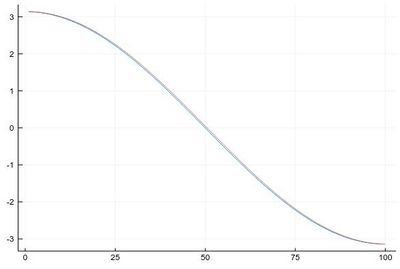
We find fairly identical-looking results:

plot([Dl(mysin,δx,"central"), Dl(mysin,δx,"left")], legend=false)

The above comparison is actually not quite correct since the lists are of different size: the left method removes one point (the last one) while the central method removes two (the first and the last one), so they shouldn't be simply overlapped but also aligned:

plot([((δx:δx:1-δx), Dl(mysin,δx,"central")),
      ((0:δx:1-δx), Dl(mysin,δx,"left"))]
    , legend=false)

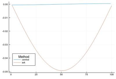
This error is actually quite large if looked at properly:

plot([
        Dl(mysin,δx,"central")-[pi*cos(pi*i) for i in δx:δx:1-δx], 
        Dl(mysin,δx,"left")-[pi*cos(pi*i) for i in 0:δx:1-δx]
    ], legendtitle="Method", legend=:bottomleft, label=["central" "left"])

This idea (and method) can be further exploited. By working out how to cancel the next-order terms, we arrive at the so-called Five-point stencil:

$$f'(x) \approx \frac{-f(x+2\epsilon)+8 f(x+\epsilon)-8 f(x-\epsilon)+f(x-2\epsilon)}{12\epsilon}$$

which we can add to our function:

function Dl(f, δx, method="central")
    if method=="left"
        diff(f)/δx
    elseif method=="central"
        [f[i+1]-f[i-1] for i=2:length(f)-1]/(2*δx)
    elseif method=="fivepoints"
        [-f[i+2]+8f[i+1]-8f[i-1]+f[i-2] for i=3:length(f)-2]/(12*δx)        
    end
end

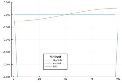
Comparing their errors:

plot([
        Dl(mysin,δx,"fivepoints")-[pi*cos(pi*i) for i in 2δx:δx:1-2δx],
        Dl(mysin,δx,"central")-[pi*cos(pi*i) for i in δx:δx:1-δx], 
        Dl(mysin,δx,"left")-[pi*cos(pi*i) for i in 0:δx:1-δx]
    ], legendtitle="Method", legend=:bottom, 
       label=["5 points" "central" "left"], ylims=(-.005,.001))

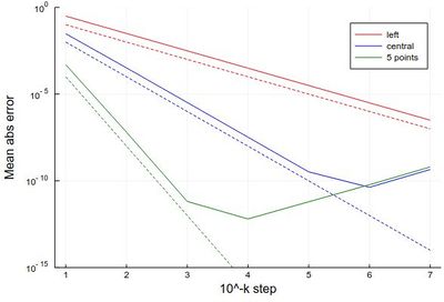
If we want a more quantitative study at the errors, we can look at how it scales for various $\epsilon$. This will allow us to look at logarithmic steps:

lδx=[10.0^(-k) for k in 1:7]
err1=[mean(abs.(Dl([sin(pi*x) for x in 0:δx:1], δx, "left")-[pi*cos(pi*x) for x in 0:δx:1-δx])) for δx in lδx]
err2=[mean(abs.(Dl([sin(pi*x) for x in 0:δx:1], δx, "central")-[pi*cos(pi*x) for x in δx:δx:1-δx])) for δx in lδx]
err3=[mean(abs.(Dl([sin(pi*x) for x in 0:δx:1], δx, "fivepoints")-[pi*cos(pi*x) for x in 2δx:δx:1-2δx])) for δx in lδx]
plot([abs.(err1) abs.(err2) abs.(err3)], 
    yscale=:log10, label=["left" "central" "5 points"], 
    xlabel="10^-k step", ylabel="Mean abs error", lc=[:red :blue :green])
plot!([x->10.0^(-x) x->10.0^(-2x) x->10.0^(-4x)],1,7,
yscale=:log10, ylims=(10^(-15),1), lc=[:red :blue :green], ls=:dash, label=["" "" ""])

with the beautiful result:

As one can see, the best method worsens for $\epsilon<10^{-4}$ so it will actually work better (and faster) for not too small an $\epsilon$.