This wikilog article is a draft, it was not published yet.
|
|
| Line 1: |
Line 1: |
| − | We could now study still other methods, such as the Backward Euler method, or Implicit Euler method. But we will instead turn to other numerical problems, namely, interpolation and extrapolation.
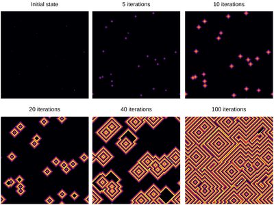
| + | <center><wz tip="Still frames for an excitable medium with a=11 and g=2">[[File:Screenshot_20210315_164359.png|400px]]</wz></center> |
| | | | |
| − | Interpolation describes the general problem of providing the value of a function which is known only for a few points, at any point which lies between other known points (if the unknown point is not "surrounded" by known points, then the problem becomes that of "extrapolation").
| + | {{WLP6}} |
| − | | + | |
| − | The simplest and also most natural method of interpolation. It has been used since immemorial times throughout history and remains a basic technique in the computer industry, which even formed a special name for it, "lerp" (also used as a verb).
| + | |
| − | | + | |
| − | The method simply consists in finding the equation for a line between two points, those which are known from the data, i.e.,
| + | |
| − | | + | |
| − | $$L(x)=f(a)+{f(b)-f(a)\over b-a}(x-a)$$
| + | |
| − | | + | |
| − | Let us assume that in the parametrization of our problem, the range of the function is the number of equally-spaced data points known and we wish to interpolate to real-valued functions. All variations of lerp will do something similar. We can then refer to the known data points $a$ and $b$ from $x$ as:
| + | |
| − | | + | |
| − | $$
| + | |
| − | \begin{align}
| + | |
| − | a&=\lfloor x\rfloor\\
| + | |
| − | b&=\lceil x\rceil
| + | |
| − | \end{align}
| + | |
| − | $$
| + | |
| − | | + | |
| − | where the floor and ceil functions are defined as follows:
| + | |
| − | | + | |
| − | <syntaxhighlight lang="python">
| + | |
| − | plot([floor, ceil], -3:.1:3, legend=false, lw=2)
| + | |
| − | </syntaxhighlight>
| + | |
| − | | + | |
| − | <center><wz tip="The floor and ceil functions (with linear interpolation causing the tilt).">[[File:Screenshot_26-03-2020_182425.jpg|400px]]</wz></center>
| + | |
| − | | + | |
| − | In this case, our linear interpolation is easily implemented. Here is some sample data:
| + | |
| − | | + | |
| − | <syntaxhighlight lang="python">
| + | |
| − | data = [sin(i) for i=0:2pi]
| + | |
| − | </syntaxhighlight>
| + | |
| − | | + | |
| − | And here is the function to "lerp" it:
| + | |
| − | | + | |
| − | <syntaxhighlight lang="python">
| + | |
| − | function lerpdata(x)
| + | |
| − | a=floor(Int,x);
| + | |
| − | b=ceil(Int,x);
| + | |
| − | data[a]+((data[b]-data[a])/(b-a))*(x-a)
| + | |
| − | end
| + | |
| − | </syntaxhighlight>
| + | |
| − | | + | |
| − | <syntaxhighlight lang="python">
| + | |
| − | scatter(data)
| + | |
| − | plot!(lerpdata,1:.01:7, lw=3, ls=:dash, legend=false)
| + | |
| − | </syntaxhighlight>
| + | |
| − | | + | |
| − | <center><wz tip="Linear interpolation of a sine.">[[File:Screenshot_26-03-2020_202110.jpg|400px]]</wz></center>
| + | |
| − | | + | |
| − | While it works well with enough points if the data has no noise, if it has, it gives disagreeable results:
| + | |
| − | | + | |
| − | <syntaxhighlight lang="python">
| + | |
| − | data = [sin(i)+rand()/5 for i=0:.1:2pi]
| + | |
| − | scatter(data)
| + | |
| − | plot!(lerpdata,1:.0001:63, lw=3, legend=false)
| + | |
| − | </syntaxhighlight>
| + | |
| − | | + | |
| − | <center><wz tip="Linear interpolation of a highly-sampled noisy sine: not a very good result.">[[File:Screenshot_26-03-2020_202640.jpg|400px]]</wz></center>
| + | |
| − | | + | |
| − | | + | |
| − | | + | |
| − | In two dimensions, linear interpolation becomes bilinear interpolations (in 3D, trilinear, etc.)
| + | |
| − | | + | |
| − | Polynomial interpolation.
| + | |
| − | | + | |
| − | Spline interpolation.
| + | |
| − | | + | |
| − | Runge's phenomenon.
| + | |
