Crash Course in Scientific Computing
III. Computer Programming
Computers are good at computing! We have seen various definitions of Euler's number $e$, of which, in particular:
$$\tag{1}e=\lim_{n\rightarrow\infty}\left(1+{1\over n}\right)^n$$
$$\tag{2}e=\sum_{k=0}^\infty{1\over k !}$$
A computer would make a great job of checking this, in particular when convergence is slow. It will also allow us to deepen this important business of convergence.
Let us compute (1): for $n=1$, this is $(1+(1/1))=2$. For $n=2$, this is $(1+(1/2))^2=9/4=2.25$. For $n=3$, this is $(1+(1/3))^3=(4/3)^3=64/27=2.\overline{370}$. Unlike computers, we get pretty tired. So we can ask the computer to do it. This is how one popular computer program, Wolfram's Mathematica, would do it:
Table[N[(1 + 1/n)^n], {n, 1, 10}]
{2., 2.25, 2.37037, 2.44141, 2.48832, 2.52163, 2.5465, 2.56578, \
2.58117, 2.59374}
It is, literally, just doing the same as we've been doing, except that it did that in 0.000041s. The command N[] in Mathematica means "numerical", since this is a symbolic program that can do both numerical (as we mainly will during this course) as well as symbolic calculations.
Back to our business: does this converge to $e\approx 2.71828$? If so, very slowly. Let us check with more points:
Table[N[(1 + 1/n)^n], {n, 1, 100}]
{2., 2.25, 2.37037, 2.44141, 2.48832, 2.52163, 2.5465, 2.56578, \
2.58117, 2.59374, 2.6042, 2.61304, 2.6206, 2.62715, 2.63288, 2.63793, \
2.64241, 2.64643, 2.65003, 2.6533, 2.65626, 2.65897, 2.66145, \
2.66373, 2.66584, 2.66778, 2.66959, 2.67128, 2.67285, 2.67432, \
2.6757, 2.67699, 2.67821, 2.67936, 2.68044, 2.68146, 2.68244, \
2.68336, 2.68423, 2.68506, 2.68586, 2.68661, 2.68733, 2.68802, \
2.68868, 2.68931, 2.68992, 2.6905, 2.69105, 2.69159, 2.6921, 2.6926, \
2.69307, 2.69353, 2.69398, 2.6944, 2.69481, 2.69521, 2.6956, 2.69597, \
2.69633, 2.69668, 2.69702, 2.69734, 2.69766, 2.69797, 2.69827, \
2.69856, 2.69884, 2.69912, 2.69938, 2.69964, 2.69989, 2.70014, \
2.70038, 2.70061, 2.70084, 2.70106, 2.70127, 2.70148, 2.70169, \
2.70189, 2.70209, 2.70228, 2.70246, 2.70264, 2.70282, 2.703, 2.70317, \
2.70333, 2.7035, 2.70365, 2.70381, 2.70396, 2.70411, 2.70426, 2.7044, \
2.70454, 2.70468, 2.70481}
This time it took 0.000449s, so still fast enough, but even the 100th number doesn't get us quite there, the 2nd decimal is still off! We can get a sense of what the computer computes by plotting it. A picture is worth a hundred numbers!
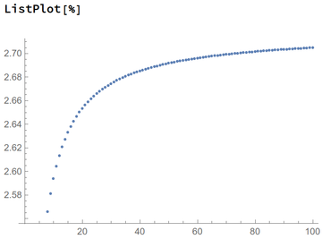
The fact that the curve still evolves (it is not horizontal), although slowly, shows that the calculation is not over. We don't have to compute all the terms though, only to take $n$ large enough, so let us see what we get with:
N[(1 + 1/1000)^1000]
2.71692
Ah ah! Well, the 2nd decimal is correct, but not the third. If we zoom as we compute, we see that convergence remains very slow:
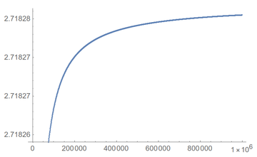
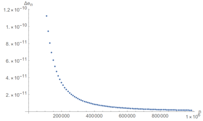
One needs $n$ as large as 743325 for a nice-looking result on screen:
A nice computer problem: which value of $n$ do we need to take so that the displayed value of $e$, i.e., to 5 decimal places, be the correct (theoretical) one? (Answer)
Let us compare with the other method, Eq. (2), which looks much more complicated since it involves a sum! for $n=1$, this is 1+1=2, the same value as before but with a sum of two. For $n=2$, this is $2+1/2=2.5$, so quite better (compare with 2.25), for $n=3$, $2.5+1/6=2.\bar 6$, so this time clearly much better (compare with 2.37 which is even worse than the $n=2$ approximation). In fact, while we needed $n=743325$ with Eq. (1), we get there with $n=8$ only using Eq. (2):
Show that $\sum_{k=0}^8(1/k!)=109\,601/40\,320=2.7182787\overline{698412}$.
Up to $n=8$ one could still compute by hand, but this becomes tedious. For a computer this is piece of cake:
le2 = Table[{n, Sum[1/k!, {k, 0, n}]}, {n, 1, 10}]
{{1, 2.}, {2, 2.5}, {3, 2.66667}, {4, 2.70833}, {5, 2.71667}, {6, 2.71806},
 {7, 2.71825}, {8, 2.71828}, {9, 2.71828}, {10, 2.71828}}
and indeed we don't see the difference, on screen. We can pass an option to Mathematica's N[] command, so that it computes to higher decimal places, including beyond machine precision, which is the maximum number that fits in the computer in native form. Let us see the result up to 25 decimal places:
le2 = Table[{n, N[Sum[1/k!, {k, 0, n}], 25]}, {n, 1, 10}]
{{1, 2.000000000000000000000000}, {2, 2.500000000000000000000000},
 {3, 2.666666666666666666666667}, {4, 2.708333333333333333333333},
 {5, 2.716666666666666666666667}, {6, 2.718055555555555555555556},
 {7, 2.718253968253968253968254}, {8, 2.718278769841269841269841},
 {9, 2.718281525573192239858907}, {10, 2.718281801146384479717813}}
as compared to:
N[E, 25]
2.718281828459045235360287
(E is $e$ in Mathematica language). Remembering that graphs show us the big picture, we can compare the convergence with this method:
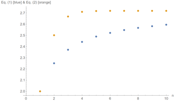
That shows that the sum is actually much more efficient. The curve quickly plateaus, we say that the result has converged and we can take it as stable with no need of further calculation.
A nice and standard way to check convergence is to compute the difference of successive terms. The speed at which this goes to zero tells us how efficient or good is the convergence (if this doesn't go to zero, then it clearly doesn't converge as the results do not tend towards a unique value). This graph should convince you that one method is much faster than the other:
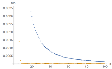
The sum of inverse factorials is so fast that we quickly lose track of its uncertainty. Convergence! We can keep an eye on it by plotting in log-scale, which means that we label our axes (only the $y$ axis in this case) not linearly but as a logarithm so that exponentials (i.e., quick changes) become line (smooth changes). If we do that, we see that convergence is very good indeed ($10^{-120}$ is a very small number) and that the single-term approximation, Eq. (1), in blue, is basically stuck:
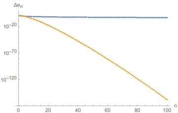
Don't get it wrong: the blue curve is also going to zero... just very slowly!
It will be a recurrent theme of the course to find out efficient numerical methods, so that we get good results quickly, involving a few resources and small numbers!
Let us turn to another nice problem involving similar calculations, namely, the Fibonacci sequence, that is formed by computing each number of the list by summing the two previous ones, $F_{n}=F_{n-1}+F_{n-2}$, starting with (for the official Fibonacci) $F_0=0$ and $F_1=1$. Clearly we have $F_2=0+1=1$, $F_3=1+1=2$, $F_4=1+2=3$, $F_5=2+3=5$, so on and so forth. The sequence thus starts:
- 0, 1, 1, 2, 3, 5, 8, 13, 21, 34, 55, 89, 144, ...
There is an encyclopedia of such integer sequences, the On-Line Encyclopedia of Integer Sequences (OEIS), which is one of the examples of good use of the Internet. There the Fibonacci appears as A000045. Read about it.
History of Science tells us that this sequence arises from a problem involving a proliferation of rabbits, a recurrent theme in mathematical modelling, which Fibonacci himself describes in 1202 in his master opus, the Liber Abaci (a book to introduce the decimal system) by asking how many pairs of rabbits are there in subsequent months given that each pair needs one month to mature and give offspring but otherwise generate one pair every month. No rabbits die. Such a simple problem can be shown by proper bookkeeping to have the solution of the sequence above. There are techniques to find a closed-form solution, but the computer would solve this readily. Or would it? Let us look at this particular implementation:
f[0]=0
f[1]=1
f[n_]:=f[n - 1] + f[n - 2]
There is a bit of syntax issues here. Mathematica requires an underscore to signify that the variable can be expanded. For us this is a detail, what we care about is that, our code indeed gives the good result:
f[5] // Timing
{0.000052, 8}
that match with Sloane's series above:
f[12] // Timing
{0.001443, 144}
but if you have a keen eye (and are good at following cues, we're not looking at the time for nothing), you'll notice something odd is going on. Let us expand on the sequence, keeping track of the times:
fib = Table[f[i] // Timing, {i, 0, 30}]
{{9.*10^-6, 0}, {2.*10^-6, 1}, {7.*10^-6, 1}, {4.*10^-6,
  2}, {6.*10^-6, 3}, {8.*10^-6, 5}, {0.000014, 8}, {0.000024,
  13}, {0.000036, 21}, {0.000059, 34}, {0.000096, 55}, {0.000153,
  89}, {0.000284, 144}, {0.000431, 233}, {0.000667, 377}, {0.001141,
  610}, {0.002197, 987}, {0.004954, 1597}, {0.006706, 2584}, {0.00735,
   4181}, {0.011941, 6765}, {0.019106, 10946}, {0.031253,
  17711}, {0.049779, 28657}, {0.081837, 46368}, {0.129615,
  75025}, {0.210993, 121393}, {0.339594, 196418}, {0.548714,
  317811}, {0.893796, 514229}, {1.45974, 832040}}
So okay, the 30th number is $F_{30}=832\,040$ obtained as $F_{29}+F_{28}=514\,229+317\,811$. But note that it took the computer a whole 1.46s to get that... which the fastest people out there would be able to . Since when are we able to compute faster than a computer?
The reason is very simple... and is one of the most dangerous pitfalls when instructing a computer: to have it do the job, but in a very inefficient, redundant and wasteful way. What's going on here, is that when we ask it to compute the sequence by involving over and over the same function, which is called "recursively" by the way, the computer goes as follows, say for
$$\begin{align} F_7&=F_6+F_5\\ &=F_5+F_4+F_4+F_3\\ &=F_4+F_3+F_3+F_2+F_3+F_2+F_2+F_1\\ &=F_3+F_2+F_2+F_1+F_2+F_1+F_1+F_0+F_2+F_1+F_1+F_0+F_1+F_0+F_1\\ &=F_2+F_1+F_1+F_0+F_1+F_0+F_1+F_1+F_0+F_1+F_1+F_0+F_1+F_0+F_1+F_1+F_0+F_1+F_0+F_1\\ &=F_1+F_0+F_1+F_1+F_0+F_1+F_0+F_1+F_1+F_0+F_1+F_1+F_0+F_1+F_0+F_1+F_1+F_0+F_1+F_0+F_1\\ &=1+0+1+1+0+1+0+1+1+0+1+1+0+1+0+1+1+0+1+0+1\\ &=13 \end{align}$$
and this is a lot of work to merely compute 5+8. So keep in mind: the computer is stupid! This is for you to do the thinking, and make it understand it doesn't need to compute over and over and over again the same thing, in this case, for instance, computing eight times $F_2$. A single time would suffice! This big problem that means that $F_{100}$ obtained in this blunt recursive way is probably out of reach of any computer, is readily removed by one innocent-looking correction, that brings back an impossible calculation into a matter of milliseconds:
f[n_] := f[n] = f[n - 1] + f[n - 2]
What we now ask the computer to do is to store in memory the result of its calculation, so that when we ask it f[n], it doesn't compute it each time, thus triggering a whole new chain of recursive calculations which will by themselves also call for more recursive calculations, resulting in this exponential slow-down, but it will check if it has it already, if not, computes it, if yes, use it straight-away.
We now look at another beautiful illustration of computer power, that revealed an unsuspected complexity in simple-looking problems, which we have already commented in our lecture on Complex Numbers. As put by Mandelbrot, take a number $c\in\mathbb{C}$ and form a sequence, a bit like the rabbits of Fibonacci, as follows:
$$z_{n+1}=(z_n+c)^2$$
with $z_0=0$. The question is, does the sequence $z_n$ diverge as $n\rightarrow\infty$? (meaning, if you remember your complex calculus, that its modulus $|z_n|$ eventually gets larger than any number you compare it to). By hand this is tedious. Let us check, as we did before, $c=1$:
We conclude with another problem, even simpler than Mandelbrot's complex (no pun intended) iterations, that will make you famous if you solve it. It is called the Collatz conjecture. Conjecture means the result is supposed, and corroborated by various types of evidence, but not demonstrated. The problem reads as follows:
Take an integer $n$ and form a sequence as follows: if the current term is even, the next term is one half of the previous term (also an integer). If the previous term is odd, the next term is 3 times the previous term plus 1.
Easy, right, especially for a computer. Collatz's conjecture is that for all $n$, the sequence will always eventually reach 1.
Let us try, first by hand:
- 1→4→2→1
- 2→1
- 3→10→5→16→8→4→2→1
well, it's true so far. Is it always true? We can never know with a computer but we can test. This requires something that starts to look like computer coding, i.e., introducing possibilities depending on the current state of affairs. This