Julia programming
m |
m |
||
| (41 intermediate revisions by one user not shown) | |||
| Line 1: | Line 1: | ||
| − | + | <center><wz tip="Still frames for an excitable medium with a=11 and g=2">[[File:Screenshot_20210315_164359.png|400px]]</wz></center> | |
| + | |||
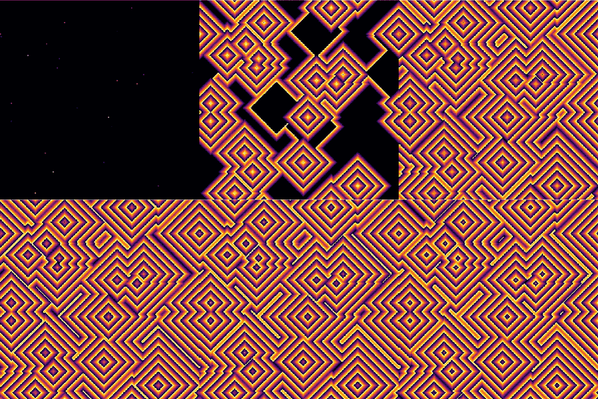
| + | Here is the same but animated: | ||
| + | |||
| + | <center><wz tip="250 iterations of the a=11 g=2 excitable model.">[[File:excitable-medium-a2-b11.gif|400px]]</wz></center> | ||
| + | |||
| + | Playing with the parameter space: | ||
| + | |||
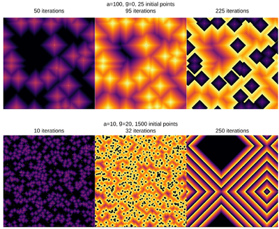
| + | <center><wz tip="Two (out of the many) configurations:">[[File:Screenshot_20210315_181551.png|400px]]</wz></center> | ||
| + | |||
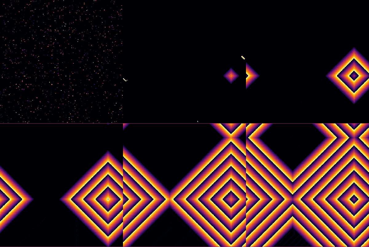
| + | And the bottom case, animated: | ||
| + | |||
| + | <center><wz tip="250 iterations of the a=10 g=20 excitable model with a lot of initially infected cells in various stages, preventing extinction.">[[File:excitable-medium-a10-b20.gif|400px]]</wz></center> | ||
| + | |||
| + | It is interesting to focus on the surviving spot. We can zoom on this area and see what is going on there. The cells have locked into this stable pattern, involving, apparently, two cells only: | ||
| + | |||
<syntaxhighlight lang="python"> | <syntaxhighlight lang="python"> | ||
| − | + | excited = @animate for i ∈ 1:30 | |
| + | excite() | ||
| + | plotspace(145, 220, 225, 300) | ||
| + | end | ||
</syntaxhighlight> | </syntaxhighlight> | ||
| − | |||
| − | |||
| − | |||
| − | |||
| − | |||
| − | |||
| − | |||
| − | |||
| − | |||
| − | |||
| − | |||
| − | |||
| − | |||
| − | + | <center><wz tip="A stable 2-cells pattern that survives in the g>a configuration by locking two neighbours with a period a+b=30.">[[File:stable-2cells-pattern.gif|400px]]</wz></center> | |
| + | |||
| + | It is interesting as well to change parameters during the simulation. This locks the patterns into some dislocated sequences which give rise to apparent cycles of stationary-evolution in space, which, however, are due to structures that formed under previous conditions of evolution. For instance, the following was obtained by iterating 50 iterations with parameters <tt>a=50 and g=25</tt> then changing <tt>g=5</tt> for 50 iterations and coming back to the initial <tt>g=25</tt> and cycling for ever: | ||
| + | |||
| + | <center><wz tip="Strange oscillations in the wake of changing parameters in mid-flight. This is an interesting optical effect due to dephasing of the wavefronts caused by dislocations in the structure following various types of evolutions.">[[File:strange-oscillations.gif|400px]]</wz></center> | ||
| + | |||
| + | There clearly appears to have two types of oscillations, one seemingly stationary in space whereas the over travels as wavefronts, that get periodically frozen. This is, however, merely an optical artifact, that can be well understood by looking at the state of the cell's evolution in time. Here is such a cut obtained in a similar configuration as the one displayed as a full density plot: | ||
| + | |||
| + | <syntaxhighlight lang="python"> | ||
| + | for i=1:75 | ||
| + | println(global iteration+=1); excite(); | ||
| + | Plots.display(plot(space[[100],:]', ylims=(0,a+g), lw=2, legend=false)) | ||
| + | end | ||
| + | </syntaxhighlight> | ||
| − | + | <center><wz tip="Slice through the cellular automaton showing two types of oscillations, as a result of dislocations: drifting and collapsing.">[[File:wavefronts-excitable-medium-cut.gif|400px]]</wz></center> | |
| − | + | One can see how the dislocations cause this alternances of drifting or collapsing evolution of the cell states. | |
| − | + | Clearly there are many variations and configurations to explore, this is barely scratching the surface. Instead of delving further into this model, we turn to the most famous and also more impressive Hodgepodge machine. | |
| − | + | {{WLP6}} | |
Latest revision as of 21:51, 15 March 2021
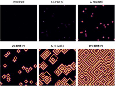
Here is the same but animated:
Playing with the parameter space:
And the bottom case, animated:
It is interesting to focus on the surviving spot. We can zoom on this area and see what is going on there. The cells have locked into this stable pattern, involving, apparently, two cells only:
excited = @animate for i ∈ 1:30
           excite()
           plotspace(145, 220, 225, 300)
       end
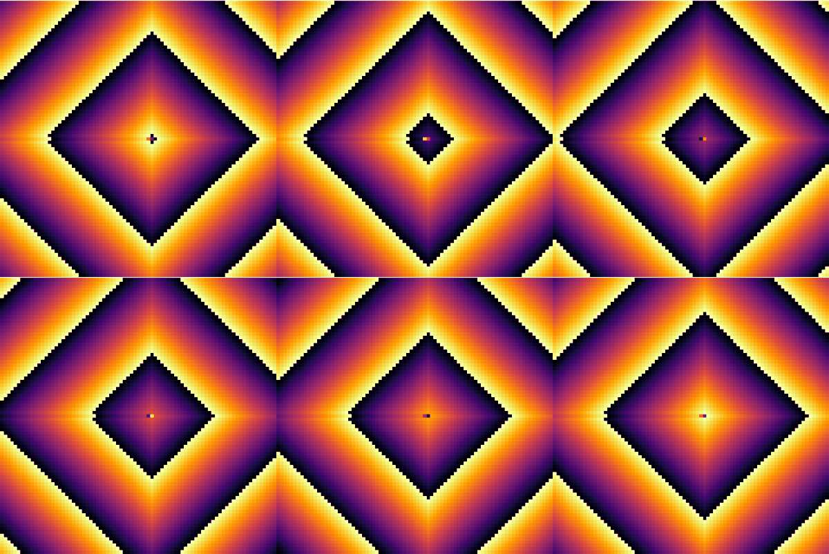
It is interesting as well to change parameters during the simulation. This locks the patterns into some dislocated sequences which give rise to apparent cycles of stationary-evolution in space, which, however, are due to structures that formed under previous conditions of evolution. For instance, the following was obtained by iterating 50 iterations with parameters a=50 and g=25 then changing g=5 for 50 iterations and coming back to the initial g=25 and cycling for ever:
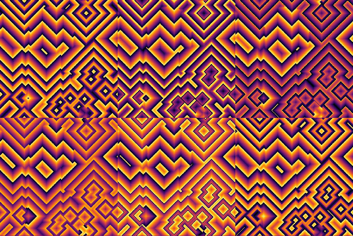
There clearly appears to have two types of oscillations, one seemingly stationary in space whereas the over travels as wavefronts, that get periodically frozen. This is, however, merely an optical artifact, that can be well understood by looking at the state of the cell's evolution in time. Here is such a cut obtained in a similar configuration as the one displayed as a full density plot:
for i=1:75
   println(global iteration+=1); excite();
   Plots.display(plot(space[[100],:]', ylims=(0,a+g), lw=2, legend=false))
end
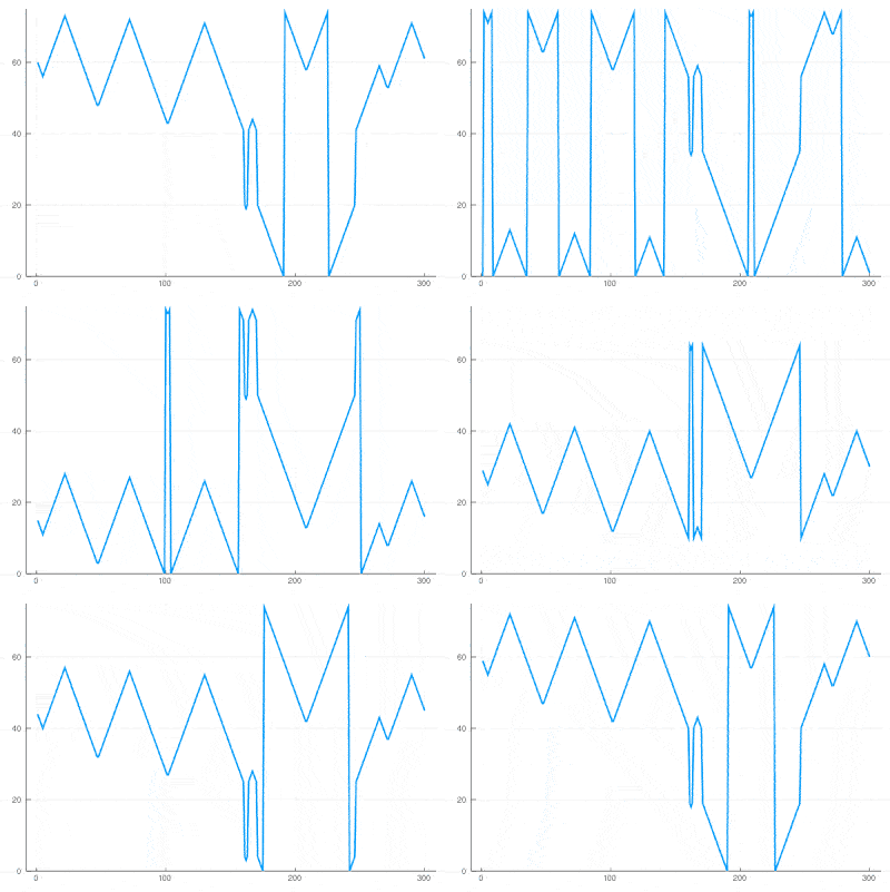
One can see how the dislocations cause this alternances of drifting or collapsing evolution of the cell states.
Clearly there are many variations and configurations to explore, this is barely scratching the surface. Instead of delving further into this model, we turn to the most famous and also more impressive Hodgepodge machine.