Revision as of 08:39, 22 March 2021

Crash Course in Scientific Computing

XIII. Root Finding

another typical numerical method: a root-finding algorithm. We used a so-called bisection method previously when generating our own random numbers, which is easy to implement but not very efficient. A simple but good improvement is the Newton–Raphson method (Newton used it for the particular case of polynomials; Raphson extended it to arbitrary functions). The idea is to start with a blind guess $x_0$ around the solution and replace the real function $f(x)$ by a linear approximation with the same slope at $x_0$, i.e., $h(x)=f'(x_0)x+\beta$ with $\beta$ such that $h(x_0)=f(x_0)$ which yields

$$h(x)=f'(x_0)[x-x_0]+f(x_0)$$

Now a better guess for the zero is found by solving $h(x)=0$ which has solution $x=x_0-(f(x_0)/f'(x_0))$. Of course the procedure can be iterated so the algorithm gives us the always better approximations:

$$x_{n+1}=x_n-{f(x_n)\over f'(x_n)}\,.$$

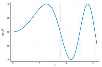
Let us find the zeros of $f(x)=\sin(x^2)$ between 0 and $\pi$. It's good to know beforehand the sort of results we expect (we added vertical lines by eye):

psin2=plot(x->sin(x^2), 0, π,
ylabel=L"\sin(x^2)",xlabel=L"x",lw=3,
legend=false)
vline!([0, 1.77, 2.51, 3.07], line = (:red, :dash, 1))
hline!([0], line = (:black, :dot, .75))

The formula gives us:

$$x_{n+1}=x_n-{\sin x_n^2\over 2x_n\cos x_n^2}$$

We can write a function that takes $f/f'$ as an input (that we have to compute ourselves) that computes such iterations until the procedure differs by less than some $\epsilon$:

function NewtonRaphson(f, x0)
    ϵ=10^-16
    x1=x0+10ϵ
    while abs(x1-x0)>ϵ
        x0=x1
        x1=x0-f(x0)
    end
    x1
end

This provides the values found in the $[0,\pi]$ interval:

lsols=[NewtonRaphson(x->sin(x^2)/(2*x*cos(x^2)), x) for x in 0:.01:π]

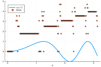
We can plot the solutions together with where was the starting point:

psin2=plot(x->sin(x^2), 0, π,
label=L"\sin(x^2)",xlabel=L"x",
legend=:bottomleft)

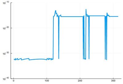
We found many, in particular some outside the $[0,\pi]$ range (this was the case when the tangent was sending us far away). We can check these are indeed all solutions:

plot(abs.(sin.(lsols.^2)), yscale=:log10, ylims=(10^-40,10^-10), legend=false)

To actually extract the values, we could use unique(), but this would return a lot of different values for the 0 zero, so we'd round this:

lsolss=sort(unique(round.(lsols,digits=10)))

These are the said solution in the sought range:

lsolss[findall(x-> 0<=x<=π, lsolss)]

5-element Array{Float64,1}:
 -0.0         
  0.0         
  1.7724538509
  2.5066282746
  3.0699801238

-0.0 and 0.0 are seen as different in julia, surely something that'll be fixed eventually. We have four solutions, as is clear from the initial graph.

There is a Roots package that has a function fzero() that achieves something similar:

fzero(x->sin(x^2), 2)

1.772453850905516