m (Created page with "= Crash Course in Scientific Computing = == XVIII. Ordinary Differential Equations: Euler & Heuhn == Let us now turn to a typical numerical problem, solving differential equa...") |
m (→Crash Course in Scientific Computing) |
||
| Line 1: | Line 1: | ||
= Crash Course in Scientific Computing = | = Crash Course in Scientific Computing = | ||
| − | == | + | == XVII. Ordinary Differential Equations: Euler & Heuhn == |
| − | Let us now turn to | + | Let us now turn to one of the most wanted tasks of scientific computing: solving differential equations. What a differential equation is in the first place is part of our Mathematics lectures and we refer you to that to get a refresher, but in a nutshell, we concern ourselves with equations of the type: |
$$\label{eq:ODE1} y'(t)=f(t,y(t))$$ | $$\label{eq:ODE1} y'(t)=f(t,y(t))$$ | ||
| − | The most famous algorithm is Euler's method and the most popular the RK4 variant of the Runge–Kutta methods. In between are a variety of possible implementations, many related in some way or the other. Methods can be explicit | + | where $y$ is the unknown—what we like to call $x$ in "normal" equations—except that here $y$ is a function, not a variable that can take a single value. If it is a function of the variable $t$, one must specify the value of $y$ at all $t$ to solve this so-called Ordinary Differential Equation (ODE), as the classification goes when there is only one variable (several variables coming next). Here $f$ is another function of both the variable, or parameter, $t$ and of the "unknown" object of interest $y$. What is a function of a function? Technically this is called a "functional" and can become quite a murky business but in our case, this is just to say that we allow any tweaking and operations on the function itself, and that the derivative at each point must correspond to such an operation on the function. For instance, here is a celebrated ODE: |
| + | |||
| + | $$\label{eq:basicODE}y'(t)=-y(t)$$ | ||
| + | |||
| + | In this case $f(t,y)=-y$ (it is not "using" the variable "slot"). This says that the derivative is proportional to the magnitude of the function: the larger is the function, the steeper its slope should be. The smaller it is, the more horizontal it should be. One can already see how the $y=0$ will be an asymptote for such a function. In fact, you should by now already see that such a differential equation has an easy solution, namely, $y(t)=y(0)\exp(-t)$. The point of numerical methods is that it will allow you to solve equations that have no such easy, or even possible, closed-form expression, such as: | ||
| + | |||
| + | $$y'(t)=\sqrt{y(t)^2+t^2}$$ | ||
| + | |||
| + | In this case, one can try to reconstruct a function $y$ such that its derivative, or slope, at all times $t$, is equal to the distance of the function from the origin. Here too one can get some intuition on the solution, for instance as time passes, the slope increases so this, in contrast to the previous case, should have an explosive nature with a vertical as an asymptote. The computer will later tell us if our intuition is correct. | ||
| + | |||
| + | The most famous and straightforward algorithm is known as Euler's method (we'll start there) and the most popular is the so-called RK4 variant of the Runge–Kutta methods. In between are a large variety of possible implementations, many related in some way or the other. If you understand the main methods, you'll be fine in adapting others if they should be needed. Methods can further be classified as "explicit"—when the solution only depends on quantities already known—or "implicit", when the solution involves other unknowns which require solving additional equations. Euler's method is explicit and, as the simplest method, is also the typical starting point to introduce the basic idea of solving ODE. Not surprisingly, it is also one of the least efficient so we will have to look at other methods, such as the "Backward Euler method" which, in turn, is implicit so it'll allow us to understand how one can solve equations relying on unknown quantities! | ||
| + | |||
| + | But first with the easy Euler method: we discretize time (we'll all our variable like this to fix ideas) into steps $t_1$, $t_2$, $\cdots$, $t_n$ separated by the same interval $h$. The sought solutions at these times are denoted $y_n\equiv y(t_n)$. Back to \eqref{eq:ODE1}, approximating $y'(t)\approx (y(t+h)-y(t))/h$, we have: | ||
$$y_{n+1}=y_n+hf(t_n,y_n)$$ | $$y_{n+1}=y_n+hf(t_n,y_n)$$ | ||
| − | This is very simple since from the solution $y_n$ at time $t_n$ we can compute the solution at $t_{n+1}$. Explicitly. | + | This is very simple since from the solution $y_n$ at time $t_n$ we can compute the solution at $t_{n+1}$. Explicitly. Hence the name. |
| − | Let us solve, for instance, | + | Let us solve, for instance, Eq. \eqref{eq:basicODE} numerically, which is good not to solve the equation but to study the method itself by comparing it to the known solution: |
<syntaxhighlight lang="python"> | <syntaxhighlight lang="python"> | ||
Revision as of 11:00, 13 April 2021
Crash Course in Scientific Computing
XVII. Ordinary Differential Equations: Euler & Heuhn
Let us now turn to one of the most wanted tasks of scientific computing: solving differential equations. What a differential equation is in the first place is part of our Mathematics lectures and we refer you to that to get a refresher, but in a nutshell, we concern ourselves with equations of the type:
$$\tag{1} y'(t)=f(t,y(t))$$
where $y$ is the unknown—what we like to call $x$ in "normal" equations—except that here $y$ is a function, not a variable that can take a single value. If it is a function of the variable $t$, one must specify the value of $y$ at all $t$ to solve this so-called Ordinary Differential Equation (ODE), as the classification goes when there is only one variable (several variables coming next). Here $f$ is another function of both the variable, or parameter, $t$ and of the "unknown" object of interest $y$. What is a function of a function? Technically this is called a "functional" and can become quite a murky business but in our case, this is just to say that we allow any tweaking and operations on the function itself, and that the derivative at each point must correspond to such an operation on the function. For instance, here is a celebrated ODE:
$$\tag{2}y'(t)=-y(t)$$
In this case $f(t,y)=-y$ (it is not "using" the variable "slot"). This says that the derivative is proportional to the magnitude of the function: the larger is the function, the steeper its slope should be. The smaller it is, the more horizontal it should be. One can already see how the $y=0$ will be an asymptote for such a function. In fact, you should by now already see that such a differential equation has an easy solution, namely, $y(t)=y(0)\exp(-t)$. The point of numerical methods is that it will allow you to solve equations that have no such easy, or even possible, closed-form expression, such as:
$$y'(t)=\sqrt{y(t)^2+t^2}$$
In this case, one can try to reconstruct a function $y$ such that its derivative, or slope, at all times $t$, is equal to the distance of the function from the origin. Here too one can get some intuition on the solution, for instance as time passes, the slope increases so this, in contrast to the previous case, should have an explosive nature with a vertical as an asymptote. The computer will later tell us if our intuition is correct.
The most famous and straightforward algorithm is known as Euler's method (we'll start there) and the most popular is the so-called RK4 variant of the Runge–Kutta methods. In between are a large variety of possible implementations, many related in some way or the other. If you understand the main methods, you'll be fine in adapting others if they should be needed. Methods can further be classified as "explicit"—when the solution only depends on quantities already known—or "implicit", when the solution involves other unknowns which require solving additional equations. Euler's method is explicit and, as the simplest method, is also the typical starting point to introduce the basic idea of solving ODE. Not surprisingly, it is also one of the least efficient so we will have to look at other methods, such as the "Backward Euler method" which, in turn, is implicit so it'll allow us to understand how one can solve equations relying on unknown quantities!
But first with the easy Euler method: we discretize time (we'll all our variable like this to fix ideas) into steps $t_1$, $t_2$, $\cdots$, $t_n$ separated by the same interval $h$. The sought solutions at these times are denoted $y_n\equiv y(t_n)$. Back to (1), approximating $y'(t)\approx (y(t+h)-y(t))/h$, we have:
$$y_{n+1}=y_n+hf(t_n,y_n)$$
This is very simple since from the solution $y_n$ at time $t_n$ we can compute the solution at $t_{n+1}$. Explicitly. Hence the name.
Let us solve, for instance, Eq. (2) numerically, which is good not to solve the equation but to study the method itself by comparing it to the known solution:
npts = 100; # number of points
y=0.0*collect(1:npts); # predefine the array
h=.1; # timesteps, so total time = npts*h=10
# The differential equation to solve
function f(t,y)
    -y
end
y[1]=1; # initial condition
# The numerical method (Euler's)
for i=1:npts-1
    y[i+1]=y[i]+h*f((i-1)*h,y[i])
end
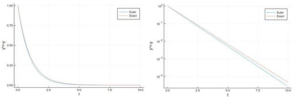
And we can now compare the numerical solution to the real one:
plot(((1:npts).-1)*h, [y[i] for i=1:npts], label="Euler", xlabel="t", ylabel="y'=-y")
plot!(x->exp(-x),0, 10, label="Exact")
Let us try the more difficult example:
$$y'={y\over 2}+2\sin(3t)\tag{3}$$
whose solution can be found with an integrating factor [1]
$$y=-{24\over37}\cos(3t)-{4\over37}\sin(3t)+\left(y(0)+{24\over 37}\right)e^{t/2}$$
In this case the differential equation is defined as:
function f(t,y)
    (y/2)+2sin(3t)
end
And the method can be quickly implemented as:
tmax=4*pi;
h=0.0001;
npts=round(Int64,tmax/h);
y=0.0*collect(1:npts);
y[1]=-24/37
for i=1:npts-1
    ti=(i-1)*h
    y[i+1]=y[i]+h*f(ti,y[i])
end
with various repetitions of
plot!(((1:npts).-1).*h, y,
    xlabel="t", ylabel="y", label="h=$(h)",
    legend=:bottomleft,ylims=(-2,.75),lw=3)
to see the effect of different time steps:
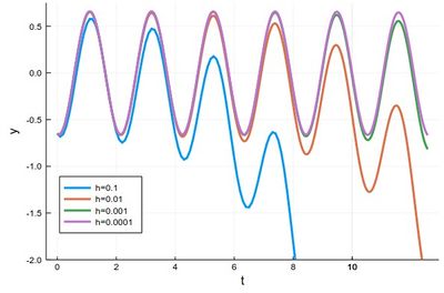
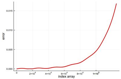
Comparing to the exact solution shows that the error gets quickly sizable, even with a lot of points:
plot(abs.([-(24/37)*cos(3t)-(4/37)*sin(3t) for t in ((1:npts).-1).*h]-y),
    lw=3, color=:red, xlabel="index array", ylabel="error", legend=false)
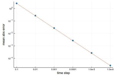
We can analyze the error in more details:
hlist=[10.0^(-k) for k=1:6];
herror=[];
for h in hlist
    npts=round(Int64,tmax/h);
    y=0.0*collect(1:npts);
    y[1]=-24/37;
    @time for i=1:npts-1
        ti=(i-1)*h
        y[i+1]=y[i]+h*f(ti,y[i])
    end
    append!(herror,mean(abs.([-(24/37)*cos(3t)-(4/37)*sin(3t) for t in ((1:npts).-1).*h]-y)))
end
produces on wulfrun2:
  0.000689 seconds (880 allocations: 15.813 KiB)
  0.003283 seconds (11.78 k allocations: 203.766 KiB)
  0.025673 seconds (136.18 k allocations: 2.270 MiB)
  0.314037 seconds (1.38 M allocations: 22.979 MiB, 1.45% gc time)
  2.519780 seconds (13.82 M allocations: 230.066 MiB, 1.00% gc time)
 26.261842 seconds (138.23 M allocations: 2.247 GiB, 2.43% gc time)
and a nice linear decay of the error with the timestep (so no-round off error, because essentially we cannot take a smaller timestep):
Euler's method works but it is not very accurate. It can be improved by considering a better estimation for the tangent. The idea is to use not the tangent of $y$ at $t_n$ only but also at $t_{n+1}$ and take the average:
$$y_{n+1}=y_n+{h\over 2}[f(t_n,y_n)+f(t_{n+1},y_{n+1})]$$
Of course, we do not know $y_{n+1}$, so the method would appear to become implicit, and we will deal with such a case later. But here, simply, we merely use Euler's method to estimate it:
$$y_{n+1}=y_n+hf(t_n,y_n)$$
so that we have an explicit formula again:
$$y_{n+1} = y_n + {h\over2} [f(t_n, y_n) + f(t_n + h, y_n + h f(t_n, y_n))]$$
This is known as Heun's method. It is one of the simplest of a class of methods called predictor-corrector algorithms (Euler's method is only a predictor method). In code:
@time for n=1:npts-1
    tn=(n-1)*h-t0;
    y[n+1]=y[n]+(h/2)*(f(tn,y[n])+f(tn+h,y[n]+h*f(tn,y[n])))
end
We can similarly compute the mean absolute error with this method:
herror=[];
for h in hlist
    npts=round(Int64,tmax/h);
    y=0.0*collect(1:npts);
    y[1]=-24/37;
    @time for n=1:npts-1
        tn=(n-1)*h;
        y[n+1]=y[n]+(h/2)*(f(tn,y[n])+f(tn+h,y[n]+h*f(tn,y[n])))
    end
    append!(herror,mean(abs.([-(24/37)*cos(3t)-(4/37)*sin(3t) for t in ((1:npts).-1).*h]-y)))
end
still on wulfrun2:
  0.000713 seconds (2.00 k allocations: 33.391 KiB)
  0.009036 seconds (23.08 k allocations: 380.391 KiB)
  0.051665 seconds (249.26 k allocations: 3.995 MiB)
  0.385209 seconds (2.51 M allocations: 40.236 MiB, 2.70% gc time)
  3.921418 seconds (25.13 M allocations: 402.639 MiB, 1.38% gc time)
 39.136207 seconds (251.33 M allocations: 3.932 GiB, 1.99% gc time)
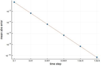
This is more resource intensive but now we get a much better $h^2$ error:
scatter(herror, xlabel="time step", ylabel="mean abs error",
    xticks=(1:6, string.(hlist)), legend=false, yscale=:log10)
plot!(x->100*herror[1]*10.0^-(2x), 1, 6, ls=:dot, lw=3)
Backward Euler method, or Implicit Euler method...