m |
m |
||
| Line 66: | Line 66: | ||
Polynomial interpolation (Lagrange). | Polynomial interpolation (Lagrange). | ||
| − | + | A great choice of interpolating polynomials is the so-called Lagrange-interpolating polynomials, which provide the unique polynomial of order $n$ to pass by the $n$ points $(x_i, y_i)$ (with $1\le i\le n$). Note that the order of the polynomial is the same as the number of points one wishes to pass through. These polynomials are obtained as a linear superposition of the Lagrange-basis polynomials: | |
| − | + | $$\ell _{j}(x)\equiv\prod _{\begin{smallmatrix}1\leq k\leq n\\k\neq j\end{smallmatrix}}{\frac {x-x_{k}}{x_{j}-x_{k}}}={\frac {(x-x_{1})}{(x_{j}-x_{1})}}\cdots {\frac {(x-x_{j-1})}{(x_{j}-x_{j-1})}}{\frac {(x-x_{j+1})}{(x_{j}-x_{j+1})}}\cdots {\frac {(x-x_{n})}{(x_{j}-x_{n})}}$$ | |
| − | Runge's phenomenon. | + | They are such that $\ell_j(x_k)=0$ for all $x_k$ with $1\le k\le n$ when $k\neq j$, otherwise $l_j(x_j)=1$. Concisely: |
| + | |||
| + | $$\ell_j(x_k)=\delta_{jk}\,.$$ | ||
| + | |||
| + | The interpolating polynomial $P_f$ of the function $f$ sampled at the points $x_k$ is then obtained as a linear superposition of the Lagrange polynomials with the values of the function as the weighting coefficients: | ||
| + | |||
| + | $$P_f(x)=\sum_{j=1}^n f(x_j)\ell_j(x)$$ | ||
| + | |||
| + | {{exstart}} | ||
| + | Given some points $(x_i, y_i)$, e.g., | ||
| + | <syntaxhighlight lang="python"> | ||
| + | xi=[1, 2, 3, 5]; | ||
| + | yi=[1, 3, 1, 2]; | ||
| + | </syntaxhighlight> | ||
| + | plot the Lagrange polynomials allowing to interpolate through all these points along with the interpolation polynomial itself. Your code should display something like this on the previous input: | ||
| + | |||
| + | <center><wz tip="The Lagrange polynomial interpolating through the given points (here four points so with a quartic polynomial).">[[File:Screenshot_20210312_153542.png|400px]]</wz></center> | ||
| + | {{anstart}} | ||
| + | <syntaxhighlight lang="python"> | ||
| + | function plotLagrange(xi, yi) | ||
| + | scatter((xi, yi), label="Data points", legend=:topleft); | ||
| + | for j=1:length(xi) | ||
| + | plot!(x->prod([(x-xi[k])/(xi[j]-xi[k]) | ||
| + | for k∈union(1:j-1,j+1:length(xi))]), | ||
| + | minimum(xi)-1, maximum(xi)+1, label="l$(j)(x)", ls=:dash) | ||
| + | end | ||
| + | plot!(x->sum([yi[j]*prod([(x-xi[k])/(xi[j]-xi[k]) | ||
| + | for k∈union(1:j-1,j+1:length(xi))]) | ||
| + | for j∈1:length(xi)]), minimum(xi)-1, maximum(xi)+1, | ||
| + | lw=3, lc=:red, label="Lagrange interpolation", xlabel="x", ylabel="f(x)") | ||
| + | end | ||
| + | </syntaxhighlight> | ||
| + | {{anstop}} | ||
| + | {{exstop}} | ||
| + | |||
| + | For instance, let us interpolate with two points (a line), at $x_1$ and $x_2=x_1+h$. The Lagrange basis in this case reads: | ||
| + | |||
| + | \begin{align} | ||
| + | l_1(x)&={x-x_2\over x_1-x_2}\\ | ||
| + | l_2(x)&={x-x_2\over x_2-x_1} | ||
| + | \end{align} | ||
| + | |||
| + | and the interpolating Lagrange polynomial becomes: | ||
| + | |||
| + | $$P_f(x)=f_1l_1(x)+f_2l_2(x)$$ | ||
| + | |||
| + | where $f_i\equiv f(x_i)$, which simplifies to (collecting $x$ and substituting $h=x_2-x_1$): | ||
| + | |||
| + | $$P_f(x)=x{f_2-f_1\over h}+(f_1+{x_1\over h}f_1-{x_1\over h}f_2)$$ | ||
| + | |||
| + | With three points, at $x_1$, $x_2=x_1+h$ and $x_3=x_1+2h$, the Lagrange polynomials read: | ||
| + | |||
| + | \begin{align} | ||
| + | l_1(x)&={x-x_2\over x_1-x_2}{x-x_3\over x_1-x_3}\\ | ||
| + | l_2(x)&={x-x_1\over x_2-x_1}{x-x_3\over x_2-x_3}\\ | ||
| + | l_3(x)&={x-x_1\over x_3-x_1}{x-x_2\over x_3-x_2} | ||
| + | \end{align} | ||
| + | |||
| + | and the Lagrange interpolating polynomial: | ||
| + | |||
| + | $$P_f(x)=f_1l_1(x)+f_2l_2(x)+f_3l_3(x)$$ | ||
| + | |||
| + | simplifies to: | ||
| + | |||
| + | $$ | ||
| + | {f_1\over 2h^2}(x^2-x(x_2+x_3)+x_2x_3) | ||
| + | -{f_2\over h^2}(x^2-x(x_1+x_3)+x_1x_3) | ||
| + | +{f_3\over 2h^2}(x^2-x(x_1+x_2)+x_1x_2) | ||
| + | $$ | ||
| + | |||
| + | |||
| + | Runge's phenomenon is the interpolation version of the French saying «''le mieux est l'ennemi du bien''» (best is the enemy of the good): adding more interpolating points to some functions results in worst results. | ||
| + | |||
| + | Other polynomial schemes. We can name, for instance, Chebyshev Interpolation or Spline interpolation. We let these to your further inquiries. | ||
{{WLP6}} | {{WLP6}} | ||
Revision as of 08:03, 4 April 2022
Crash Course in Scientific Computing
XVII. Interpolation
This page is still largely in progress.
Interpolation describes the general problem of providing the value of a function, which is known only for a few points, at any point which lies between other known points (if the unknown point is not "surrounded" by known points, then the problem becomes that of "extrapolation", next lecture).
The simplest and also most natural method of interpolation is linear interpolation, which assumes that two neighbouring points are linked by a line. It has been used since immemorial times throughout history and remains a basic technique in the computer industry, which even formed a special name for it, "lerp" (also used as a verb).
The method simply consists in finding the equation for a line between two points, those which are known from the data, i.e.,
$$L(x)=f(a)+{f(b)-f(a)\over b-a}(x-a)$$
Let us assume that in the parametrization of our problem, the range of the function is the number of equally-spaced data points known and we wish to interpolate to real-valued functions. All variations of lerp will do something similar. We can then refer to the known data points $a$ and $b$ from $x$ as:
$$ \begin{align} a&=\lfloor x\rfloor\\ b&=\lceil x\rceil \end{align} $$
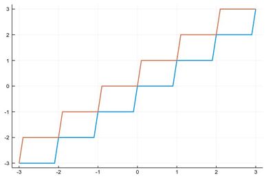
where the floor and ceil functions are defined as follows:
plot([floor, ceil], -3:.1:3, legend=false, lw=2)

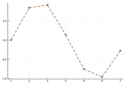
In this case, our linear interpolation is easily implemented. Here is some sample data:
data = [sin(i) for i=0:2pi]
And here is the function to "lerp" it:
function lerpdata(x)
    a=floor(Int,x);
    b=ceil(Int,x);
    data[a]+((data[b]-data[a])/(b-a))*(x-a)
end
scatter(data)
plot!(lerpdata,1:.01:7, lw=3, ls=:dash, legend=false)

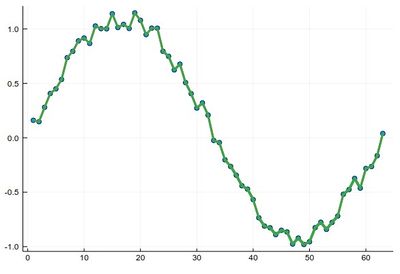
While it works well with enough points if the data has no noise, if it has, it gives disagreeable results:
data = [sin(i)+rand()/5 for i=0:.1:2pi]
scatter(data)
plot!(lerpdata,1:.0001:63, lw=3, legend=false)

In two dimensions, linear interpolation becomes bilinear interpolations (in 3D, trilinear, etc.)
Polynomial interpolation (Lagrange).
A great choice of interpolating polynomials is the so-called Lagrange-interpolating polynomials, which provide the unique polynomial of order $n$ to pass by the $n$ points $(x_i, y_i)$ (with $1\le i\le n$). Note that the order of the polynomial is the same as the number of points one wishes to pass through. These polynomials are obtained as a linear superposition of the Lagrange-basis polynomials:
$$\ell _{j}(x)\equiv\prod _{\begin{smallmatrix}1\leq k\leq n\\k\neq j\end{smallmatrix}}{\frac {x-x_{k}}{x_{j}-x_{k}}}={\frac {(x-x_{1})}{(x_{j}-x_{1})}}\cdots {\frac {(x-x_{j-1})}{(x_{j}-x_{j-1})}}{\frac {(x-x_{j+1})}{(x_{j}-x_{j+1})}}\cdots {\frac {(x-x_{n})}{(x_{j}-x_{n})}}$$
They are such that $\ell_j(x_k)=0$ for all $x_k$ with $1\le k\le n$ when $k\neq j$, otherwise $l_j(x_j)=1$. Concisely:
$$\ell_j(x_k)=\delta_{jk}\,.$$
The interpolating polynomial $P_f$ of the function $f$ sampled at the points $x_k$ is then obtained as a linear superposition of the Lagrange polynomials with the values of the function as the weighting coefficients:
$$P_f(x)=\sum_{j=1}^n f(x_j)\ell_j(x)$$
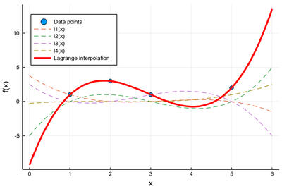
Given some points $(x_i, y_i)$, e.g.,
xi=[1, 2, 3, 5];
yi=[1, 3, 1, 2];
plot the Lagrange polynomials allowing to interpolate through all these points along with the interpolation polynomial itself. Your code should display something like this on the previous input:

function plotLagrange(xi, yi)
    scatter((xi, yi), label="Data points", legend=:topleft);
    for j=1:length(xi)
        plot!(x->prod([(x-xi[k])/(xi[j]-xi[k])
                       for k∈union(1:j-1,j+1:length(xi))]),
              minimum(xi)-1, maximum(xi)+1, label="l$(j)(x)", ls=:dash)
    end
    plot!(x->sum([yi[j]*prod([(x-xi[k])/(xi[j]-xi[k])
                              for k∈union(1:j-1,j+1:length(xi))])
                  for j∈1:length(xi)]), minimum(xi)-1, maximum(xi)+1,
          lw=3, lc=:red, label="Lagrange interpolation", xlabel="x", ylabel="f(x)")
end
For instance, let us interpolate with two points (a line), at $x_1$ and $x_2=x_1+h$. The Lagrange basis in this case reads:
\begin{align} l_1(x)&={x-x_2\over x_1-x_2}\\ l_2(x)&={x-x_2\over x_2-x_1} \end{align}
and the interpolating Lagrange polynomial becomes:
$$P_f(x)=f_1l_1(x)+f_2l_2(x)$$
where $f_i\equiv f(x_i)$, which simplifies to (collecting $x$ and substituting $h=x_2-x_1$):
$$P_f(x)=x{f_2-f_1\over h}+(f_1+{x_1\over h}f_1-{x_1\over h}f_2)$$
With three points, at $x_1$, $x_2=x_1+h$ and $x_3=x_1+2h$, the Lagrange polynomials read:
\begin{align} l_1(x)&={x-x_2\over x_1-x_2}{x-x_3\over x_1-x_3}\\ l_2(x)&={x-x_1\over x_2-x_1}{x-x_3\over x_2-x_3}\\ l_3(x)&={x-x_1\over x_3-x_1}{x-x_2\over x_3-x_2} \end{align}
and the Lagrange interpolating polynomial:
$$P_f(x)=f_1l_1(x)+f_2l_2(x)+f_3l_3(x)$$
simplifies to:
$$ {f_1\over 2h^2}(x^2-x(x_2+x_3)+x_2x_3) -{f_2\over h^2}(x^2-x(x_1+x_3)+x_1x_3) +{f_3\over 2h^2}(x^2-x(x_1+x_2)+x_1x_2) $$
Runge's phenomenon is the interpolation version of the French saying «le mieux est l'ennemi du bien» (best is the enemy of the good): adding more interpolating points to some functions results in worst results.
Other polynomial schemes. We can name, for instance, Chebyshev Interpolation or Spline interpolation. We let these to your further inquiries.