Crash Course in Scientific Computing

XIV. Derivatives

How about the reverse process, i.e., derivation. We can use the diff command that computes finite differences:

diff(1:.5:10)

returns an array of 18 elements, all equal to 0.5. In this way, it is easy to compute a finite-difference derivative:

plot(diff([sin(pi*x) for x=0:.01:1])./.01)

This is a cosine. Importantly for numerical methods, one should look for simple tricks that maximise numerical accuracies. The idea behind differentiation comes from Taylor expansion:

\begin{equation} \tag{1} f(x\pm\epsilon)=f(x)\pm\epsilon f'(x)+{\epsilon^2\over2} f''(x)\pm{\epsilon^3\over6} f'''(x)+o(\epsilon^4) \end{equation}

that we wrote for both $\pm\epsilon$, and using the $o$-notation to mean that terms we neglected are of the order of $\epsilon^4$. From this, one can get an obvious numerical approximation for the derivative

$$f'(x)\approx{f(x\pm\epsilon)-f(x)\over\epsilon}+o(\epsilon)$$

meaning we can expect an error of the order of $\epsilon$ with this method. Observe however how one can sneakily cancel the $\epsilon^2$ term from (1) by subtracting $f(x-\epsilon)$ from $f(x+\epsilon)$:

$$f(x+\epsilon)-f(x-\epsilon)=2\epsilon f'(x)+{\epsilon^3\over 3}{f'''(x)}+o(\epsilon^4)$$

so that we have a much better approximation by computing with this slight variation:

$$f'(x)={f(x+\epsilon)-f(x-\epsilon)\over 2\epsilon}+o(\epsilon^2)$$

since $\epsilon^2\ll\epsilon$. The computational cost is the same, the numerical gain is considerable. Let's write a function. We'll it call Dl for "Differentiate list":

function Dl(f, δx, method="central")
    if method=="left"
        diff(f)/δx
    elseif method=="central"
        [f[i+1]-f[i-1] for i=2:length(f)-1]/(2*δx)
    end
end

Let us compare the two methods for

δx=0.1;
mysin=[sin(pi*x) for x in 0:δx:1]

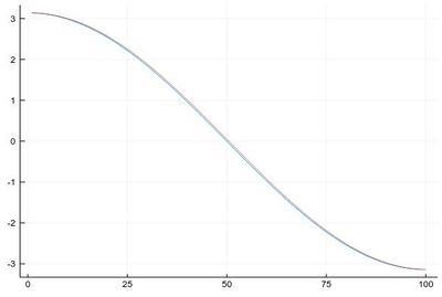
We find fairly identical-looking results:

plot([Dl(mysin,δx,"central"), Dl(mysin,δx,"left")], legend=false)

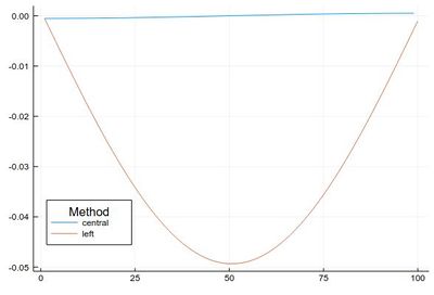
This error is actually quite large if looked at properly: (note the comparison to lists of different size, the central method removes two points)

plot([
        Dl(mysin,δx,"central")-[pi*cos(pi*i) for i in δx:δx:1-δx], 
        Dl(mysin,δx,"left")-[pi*cos(pi*i) for i in 0:δx:1-δx]
    ], legendtitle="Method", legend=:bottomleft, label=["central" "left"])

This idea (and method) can be further exploited. By working out how to cancel the next-order terms, we arrive at the so-called Five-point stencil:

$$f'(x) \approx \frac{-f(x+2\epsilon)+8 f(x+\epsilon)-8 f(x-\epsilon)+f(x-2\epsilon)}{12\epsilon}$$

which we can add to our function:

function Dl(f, δx, method="central")
    if method=="left"
        diff(f)/δx
    elseif method=="central"
        [f[i+1]-f[i-1] for i=2:length(f)-1]/(2*δx)
    elseif method=="fivepoints"
        [-f[i+2]+8f[i+1]-8f[i-1]+f[i-2] for i=3:length(f)-2]/(12*δx)        
    end
end

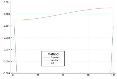
Comparing their errors:

plot([
        Dl(mysin,δx,"fivepoints")-[pi*cos(pi*i) for i in 2δx:δx:1-2δx],
        Dl(mysin,δx,"central")-[pi*cos(pi*i) for i in δx:δx:1-δx], 
        Dl(mysin,δx,"left")-[pi*cos(pi*i) for i in 0:δx:1-δx]
    ], legendtitle="Method", legend=:bottom, 
       label=["5 points" "central" "left"], ylims=(-.005,.001))

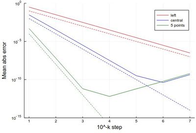
If we want a more quantitative study at the errors, we can look at how it scales for various $\epsilon$. This will allow us to look at logarithmic steps:

lδx=[10.0^(-k) for k in 1:7]
err1=[mean(abs.(Dl([sin(pi*x) for x in 0:δx:1], δx, "left")-[pi*cos(pi*x) for x in 0:δx:1-δx])) for δx in lδx]
err2=[mean(abs.(Dl([sin(pi*x) for x in 0:δx:1], δx, "central")-[pi*cos(pi*x) for x in δx:δx:1-δx])) for δx in lδx]
err3=[mean(abs.(Dl([sin(pi*x) for x in 0:δx:1], δx, "fivepoints")-[pi*cos(pi*x) for x in 2δx:δx:1-2δx])) for δx in lδx]
plot([abs.(err1) abs.(err2) abs.(err3)], 
    yscale=:log10, label=["left" "central" "5 points"], 
    xlabel="10^-k step", ylabel="Mean abs error", lc=[:red :blue :green])
plot!([x->10.0^(-x) x->10.0^(-2x) x->10.0^(-4x)],1,7,
yscale=:log10, ylims=(10^(-15),1), lc=[:red :blue :green], ls=:dash, label=["" "" ""])

with the beautiful result:

As one can see, the best method worsens for $\epsilon<10^{-4}$ so it will actually work better (and faster) for not too small an $\epsilon$.