Crash Course in Scientific Computing
XV. Derivatives
Pax: Hey, Cleve, you ought to blog about that complex step algorithm you invented.
Me: What are you talking about?
Pax: You know, differentiation using complex arithmetic. It's hot stuff. We're using it in SimBiology.
Me: I don't remember inventing any complex step differentiation algorithm.
Pax: Well, an old paper of yours is referenced. Lots of people are using it today.
We now turn to the reverse process of last lecture's topic (it was on integrals), i.e., derivation. While in pure (pen-and-paper) Maths, differentiation is typically easier than integration, numerically, the difficulty is reversed. This is because integration as summing patches of the functions works well with basic continuity properties (e.g., not be discontinuous) while differentiation requires stronger properties, in particular the so-called Lipschitz continuity that limits how fast the function, even though continuous, can change. It also is very fragile to dividing by small numbers although a fairly recent "hack" against has been proposed by making a detour into the complex plane, as we shall see.
The basic idea behind differentiation comes from Taylor expansion:
\begin{equation} \tag{1} f(x\pm\epsilon)=f(x)\pm\epsilon f'(x)+{\epsilon^2\over2} f''(x)\pm{\epsilon^3\over6} f'''(x)+o(\epsilon^4) \end{equation}
that we wrote for both $\pm\epsilon$, and using the $o$-notation to mean that terms we neglected are of the order of $\epsilon^4$. From this, one can get the most obvious and natural numerical approximation for the derivative
$$f'(x)\approx\pm{f(x\pm\epsilon)-f(x)\over\epsilon}+o(\epsilon)$$
meaning we can expect an error of the order of $\epsilon$ with this method (namely $\approx{\epsilon\over 2}f''(x)$). We also see here one problem of numerical derivatives, which is that they imply dividing by a small number $h$, which is notoriously unstable and problematic. On the other hand, the numerator itself is a simple, so-called finite difference. We can use the diff command to computes finite differences:
diff(1:.5:10)
returns an array of 18 elements, all equal to 0.5. In this way, it is easy to compute a finite-difference derivative:
plot(diff([sin(pi*x) for x=0:.01:1])./.01)
This is a cosine. Importantly for numerical methods, one should look for simple tricks that maximise numerical accuracies. Observe, indeed, how one can sneakily cancel the $\epsilon^2$ term from (1) by subtracting $f(x-\epsilon)$ from $f(x+\epsilon)$:
$$f(x+\epsilon)-f(x-\epsilon)=2\epsilon f'(x)+{\epsilon^3\over 3}{f'''(x)}+o(\epsilon^3)$$
so that we have a much better approximation by computing with this slight variation:
$$f'(x)={f(x+\epsilon)-f(x-\epsilon)\over 2\epsilon}+o(\epsilon^2)$$
since $\epsilon^2\ll\epsilon$. The computational cost is the same, the numerical gain is considerable. Let's write a function. We'll it call Dl for "Differentiate list":
function Dl(f, δx, method="central")
    if method=="left"
        diff(f)/δx
    elseif method=="central"
        [f[i+1]-f[i-1] for i=2:length(f)-1]/(2*δx)
    end
end
Let us compare the two methods for
δx=0.01;
mysin=[sin(pi*x) for x in 0:δx:1]
We find fairly identical-looking results:
plot([Dl(mysin,δx,"central"), Dl(mysin,δx,"left")], legend=false)
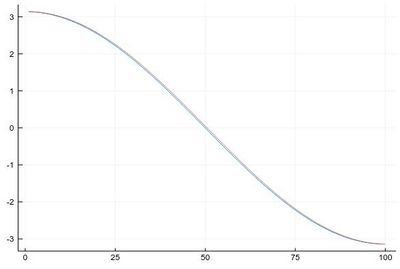
The above comparison is actually not quite correct since the lists are of different size: the left method removes one point (the last one) while the central method removes two (the first and the last one), so they shouldn't be simply overlapped but also aligned; the difference would become significative with larger steps:
δx=0.1;
plot([((δx:δx:1-δx), Dl(mysin,δx,"central")),
      ((0:δx:1-δx), Dl(mysin,δx,"left"))],
      legend=false)

plot!(x-> pi*cos(pi*x), 0:.01:1, lc=:red, ls=:dashdotdot, la=.5, lw=3,
             xlabel="x", ylabel="sin(pi x)'", label="exact", dpi=200)
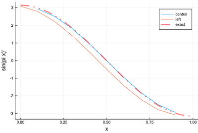
Derivatives of $\sin(\pi x)$ with a large step: the central method is incredibly accurate!
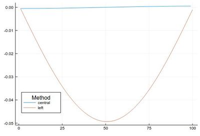
Even with a small step, δx=0.01, this error is actually quite large if looked at properly:
plot([
        Dl(mysin,δx,"central")-[pi*cos(pi*i) for i in δx:δx:1-δx],
        Dl(mysin,δx,"left")-[pi*cos(pi*i) for i in 0:δx:1-δx]
    ], legendtitle="Method", legend=:bottomleft, label=["central" "left"])
One is also often interested in higher-order derivative. One would be tempted in using iterated derivations, which is, after all, the mathematical definition: $f''=(f')'$, so:
Dl(Dl(mysin, δx), δx)
That would work but it is better to implement this iteration at the core of the numerical method, rather than to iterate it from the outset, which will accumulate errors and multiply the number of operations. Here is a simple (also central) finite-difference formula:
$$f''(x)\approx{\frac {{\frac {f(x+h)-f(x)}{h}}-{\frac {f(x)-f(x-h)}{h}}}{h}}={\frac {f(x+h)-2f(x)+f(x-h)}{h^{2}}}$$
that we can implement as:
function Dl(f, δx, method="central", n=1)
    if n==1
        if method=="left"
            diff(f)/δx
        elseif method=="central"
            [f[i+1]-f[i-1] for i=2:length(f)-1]/(2*δx)
        end
    elseif n==2
        if method=="central"
            [f[i+1]-2f[i]+f[i-1] for i=2:length(f)-1]/(δx^2)
        else
            println("Sorry, method not available.")
        end
    end
end
which both give apparently similar-looking results:
bigsin=[sin(x) for x in 0:δx:2pi]
plot([Dl(Dl(bigsin, δx), δx), Dl(bigsin, δx, "central", 2)],
                    label=["(f')'" "f''"], legend=:topleft)
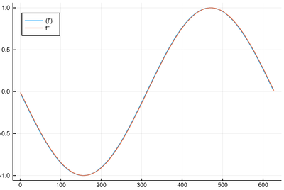
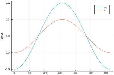
The error, in this case, is not very dramatic but it is significantly still better to use the second-order derivative once:
julia> plot([Dl(Dl(bigsin, δx), δx)-[-sin(x) for x in 0:δx:2pi-4δx],
             Dl(bigsin, δx, "central", 2)-[-sin(x) for x in 0:δx:2pi-2δx]],
             label=["(f')'" "f''"], ylabel="error")
This idea of finding how to best combine finite differences of the function to approximate with the smallest possible error its derivative to a given order can be generalized in a similar way than we did for integration, namely, using Lagrange interpolation polynomials. We will apply it directly to a 5-order polynomial as lowest orders reproduce the results we already got from direct methods:
Show that derivating Lagrange polynomials to order 2, 3 and 4 reproduce finite-difference results in different combinations (e.g., forward).
We use, therefore, the five points $x_j$ with integer $j$ such that $-2\le j\le 2$ and we shall look at the central method, which is the most common, so taking eventually $x=x_0$. For any $x$, the interpolation to order 5 reads:
$$P_f(x)\equiv\sum_{j=-2}^2f(x_j)\ell_j(x)$$
The Lagrange polynomial remains, after all, a polynomial, so its derivative is in principle straightforward.
Show that the derivative of the Lagrange polynomial is given by:
$${\ell_{j}'(x)=\sum_{i\neq j}\left[{\frac {1}{x_{j}-x_{i}}}\prod_{m\neq i,j}{\frac {x-x_{m}}{x_{j}-x_{m}}}\right]}\tag{2}\,.$$
Write a piece of code to plot these derivatives and check it against numerical differentiation of the Lagrange polynomials.
The calculation simplifies a lot by taking the logarithm of both sides: \begin{equation} \ln\ell_{j}(x)=\sum_{k\neq j}\ln{x-x_k\over x_j-x_k} \end{equation}
in which case the products turns into a trivial sum of linear functions:
\begin{equation} \left(\ln\ell_{j}(x)\right)'={\ell_j(x)'\over\ell_j(x)}=\sum_{k\neq j}\left(\ln{x-x_k\over x_j-x_k}\right)' =\sum_{k\neq j}{1\over x-x_k}\,. \end{equation}
so that the result is obtained immediately as:
\begin{equation} \ell_j(x)'=\ell_j(x)\sum_{k\neq j}{1\over x-x_k}\,. \end{equation}
This is, in fact, a deceivingly simple result, which appears to be ill-defined at all $x\neq x_j$, although it is not as it implies cancellations of terms which lead to some 0/0 indeterminacy if not explicitly simplified. Expanding $\ell_j(x)$ on the right-hand side and simplifying these terms, we find:
\begin{align} \ell_j(x)'&=\sum_{i\neq j}\prod_{m\neq j}{1\over x-x_i}{\frac {x-x_m}{x_j-x_m}}\,,\\ &=\sum_{i\neq j}{1\over x_j-x_i}\prod_{m\neq j,i}{\frac {x-x_m}{x_j-x_m}}\,,\\ \end{align}
which is the expression given.
and thus, its derivative is:
$$P_f(x)'\equiv\sum_{j=-2}^2f(x_j)\sum_{i\neq j}\left[{\frac {1}{x_{j}-x_{i}}}\prod_{m\neq i,j}{\frac {x-x_{m}}{x_{j}-x_{m}}}\right]$$
that, for clarity, we can spell out for the first summation and also evaluate at $x=x_0$ (other points of the grids are possible and would give other finite difference formulas for derivatives):
\begin{align} P_f(x_0)'=f(x_{-2})\sum_{i\neq-2}&\left[{\frac {1}{x_{-2}-x_{i}}}\prod_{m\neq i,-2}{\frac {x_0-x_{m}}{x_{-2}-x_{m}}}\right]\\ +f(x_{-1})\sum_{i\neq-1}&\left[{\frac {1}{x_{-1}-x_{i}}}\prod_{m\neq i,-1}{\frac {x_0-x_{m}}{x_{-1}-x_{m}}}\right]\\ +f(x_{0})\sum_{i\neq0}&\left[{\frac {1}{x_{0}-x_{i}}}\prod_{m\neq i,0}{\frac {x_0-x_{m}}{x_{0}-x_{m}}}\right]\\ +f(x_{1})\sum_{i\neq1}&\left[{\frac {1}{x_{1}-x_{i}}}\prod_{m\neq i,1}{\frac {x_0-x_{m}}{x_{1}-x_{m}}}\right]\\ +f(x_{2})\sum_{i\neq2}&\left[{\frac {1}{x_{2}-x_{i}}}\prod_{m\neq i,2}{\frac {x_0-x_{m}}{x_{2}-x_{m}}}\right] \end{align}
Now, in each case, the product will cancel unless $m\neq 0$ which for all except the middle line is possible only if $i$ itself is~0, so that the expression simplifies to:
\begin{align} P_f(x_0)'=f(x_{-2})&\left[{\frac {1}{x_{-2}-x_{0}}}\prod_{m\neq 0,-2}{\frac {x_0-x_{m}}{x_{-2}-x_{m}}}\right]\\ +f(x_{-1})&\left[{\frac {1}{x_{-1}-x_{0}}}\prod_{m\neq 0,-1}{\frac {x_0-x_{m}}{x_{-1}-x_{m}}}\right]\\ +f(x_{0})&\sum_{i\neq0}{\frac {1}{x_{0}-x_{i}}}\\ +f(x_{1})&\left[{\frac {1}{x_{1}-x_{0}}}\prod_{m\neq 0,1}{\frac {x_0-x_{m}}{x_{1}-x_{m}}}\right]\\ +f(x_{2})&\left[{\frac {1}{x_{2}-x_{0}}}\prod_{m\neq 0,2}{\frac {x_0-x_{m}}{x_{2}-x_{m}}}\right] \end{align}
which is now just a matter of evaluating on a grid which, typically, one would take with equidistant points around $x_0$, namely, $x_k=x_0+kh$ for $-2\le k\le 2$. It is an easy exercise (and good practice in keeping track of several indices) to show that this results in the so-called Five-point stencil formula:
Show that on a grid with five points such that $x_{-2}=x_0-2h$, $x_{-1}=x_0-h$, $x_1=x_0+h$ and $x_2=x_0+2h$, one finds from the 5-th order Lagrange-polynomial interpolation the following central-formula for the derivative:
$$f'(x_0) \approx \frac{f(x-2h)-8 f(x-h)+8 f(x+h)-f(x+2h)}{12h}\,.$$
This is just a matter of careful substitutions and simplifications. One finds: \begin{align} P_f(x_0)'=f(x_{-2})&{1\over x_{-2}-x_0}{x_0-x_{-1}\over x_{-2}-x_{-1}}{x_0-x_{1}\over x_{-2}-x_{1}}{x_0-x_{2}\over x_{-2}-x_{2}}\\ +f(x_{-1})&{1\over x_{-1}-x_0}{x_0-x_{-2}\over x_{-1}-x_{-2}}{x_0-x_{1}\over x_{-1}-x_{1}}{x_0-x_{2}\over x_{-1}-x_{2}}\\ +f(x_{0})&\left({1\over x_0-x_{-2}}+{1\over x_0-x_{-1}}+{1\over x_0-x_{1}}+{1\over x_0-x_{2}}\right)\\ +f(x_{1})&{1\over x_{1}-x_0}{x_0-x_{-2}\over x_{1}-x_{-2}}{x_0-x_{-1}\over x_{1}-x_{-1}}{x_0-x_{2}\over x_{1}-x_{2}}\\ +f(x_{2})&{1\over x_{2}-x_0}{x_0-x_{-2}\over x_{2}-x_{-2}}{x_0-x_{-1}\over x_{2}-x_{-1}}{x_0-x_{1}\over x_{2}-x_{1}}\\ =f(x_{-2})&{1\over-2h}{h\over-h}{-h\over-3h}{-2h\over-4h}\\ +f(x_{-1})&{1\over-h}{2h\over h}{-h\over-2h}{-2h\over-3h}\\ +f(x_0)&\left({1\over2h}+{1\over h}+{1\over-h}+{1\over-2h}\right)\\ +f(x_1)&{1\over h}{2h\over3h}{h\over2h}{-2h\over-h}\\ +f(x_2)&{1\over2h}{2h\over4h}{h\over3h}{-h\over h} \end{align} which further simplifies to the expression given.
Note that although the five-point formula involves four coefficients, it really involves five points in interpolating the function, since it pins the interpolating polynomial also at $f(x_0)$ even if, in the final result, the value of the function there does not contribute to its derivative. We can add this formula to our numerical-derivative function:
function Dl(f, δx, method="central")
    if method=="left"
        diff(f)/δx
    elseif method=="central"
        [f[i+1]-f[i-1] for i=2:length(f)-1]/(2*δx)
    elseif method=="fivepoints"
        [-f[i+2]+8f[i+1]-8f[i-1]+f[i-2] for i=3:length(f)-2]/(12*δx)
    end
end
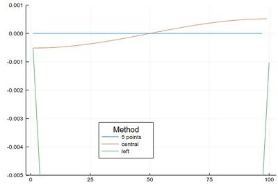
Comparing their errors:
plot([
        Dl(mysin,δx,"fivepoints")-[pi*cos(pi*i) for i in 2δx:δx:1-2δx],
        Dl(mysin,δx,"central")-[pi*cos(pi*i) for i in δx:δx:1-δx],
        Dl(mysin,δx,"left")-[pi*cos(pi*i) for i in 0:δx:1-δx]
    ], legendtitle="Method", legend=:bottom,
       label=["5 points" "central" "left"], ylims=(-.005,.001))
The same method can be generalized to higher orders of the derivative. We then need to invoke the expression for the $n$th derivative of the Lagrange interpolating polynomials, which can be done easily by recursion. For instance:
Show that the second-order derivative of the Lagrange basis polynomial is given by: $$\ell_i(x)'' =\sum_{l\ne i}\frac{1}{x_i-x_l}\left( \sum_{m\ne i,l}\frac{1}{x_i-x_m}\prod_{k\ne i,l,m}\frac{x-x_k}{x_i-x_k}\right)\,.$$ Use this result to obtain a five-point stencil finite-difference formula for $f''$. By recurrence, obtain $\ell_i(x)'''$ and use it to obtain a five-point stencil finite-difference formula for $f''$.
Using this method, one can tabulate a list (of which the previous exercise should give you two lines) for, say, the central-method (equal number of points on both sides of the point at which the derivative is being calculated) on an equidistant grid. This one comes from the paper which first settled down the simplified procedure:[1]
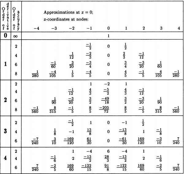
Tables can also be found online, e.g., on the Wikipedia. The derivative at $x_0$ is approximated by taking the sum of the function at the points given (central finite-difference) weighted by the corresponding coefficients and divided by the grid-step to the power of the order of the derivative. For instance:
\begin{equation} f^{(4)}(x_0)\approx{ {-1\over6}f(x_{-3}) +2f(x_{-2}) +{-13\over2}f(x_{-1}) +{28\over3}f(x_0) +{-13\over2}f(x_{1}) +2f(x_{2}) {-1\over6}f(x_{3}) \over h^4} \end{equation}
We can implement, say, all the first-order derivatives from this table (now referring to the method by its order, and using different ways to write down the formulas, e.g., with grouping of the same coefficients, for the order 8 one):
function Dl(f, δx, order=4)
    if order==1
        diff(f)/δx
    elseif order==2
        [f[i+1]-f[i-1] for i=2:length(f)-1]/(2*δx)
    elseif order==4
        [f[i-2]-8f[i-1]+8f[i+1]-f[i+2] for i=3:length(f)-2]/(12*δx)
    elseif order==6
        [-f[i-3]+9f[i-2]-45f[i-1]+45f[i+1]-9f[i+2]+f[i+3] for i=4:length(f)-3]/(60*δx)
    elseif order==8
        [(1/280)*(f[i-4]-f[i+4])-(4/105)*(f[i-3]-f[i+3])+(1/5)*(f[i-2]-f[i+2])-(4/5)*(f[i-1]-f[i+1]) for i=5:length(f)-4]/δx
    end
end
We can now have a more quantitative look at the errors and how it scales with the timestep.
p=plot();
for i in 1:5
    err=[mean(abs.(Dl([sin(pi*x/4) for x in 0:δx:5], δx, lo[i])
                     -[(pi/4)*cos(pi*x/4) for x in (i-1)*δx:δx:5-(i==1 ? 1 : (i-1))*δx])) for δx in lδx]
    plot!(abs.(err), yscale=:log10, label="order $(lo[i])", lc=palette(:default)[i])
    scatter!(abs.(err), yscale=:log10, label="", mc=palette(:default)[i], m=2)
end
for i in 1:5
    plot!(x->2.0^(-lo[i]*x)/3^lo[i],1,20, yscale=:log10, ylims=(10^(-16),1), lc=:black, ls=:dash, label="")
end
plot!(xticks = (1:length(lδx), ["\$2^{-$(k)}\$" for k∈1:length(lδx)]), dpi=360,
      xformatter = :latex, xlabel = "Step in derivative", ylabel="Error")
p
with the beautiful result, matched against the theoretical slope (in dashed):
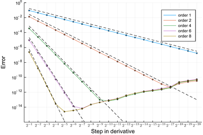
where we see that, even on a base-2 grid, the error now irremediably increases as the time-step decreases, illustrating the already commented greater sensibility of the derivative than the integral, which was staying pinned at the machine precision. Here, instead, as we try to improve the algorithmic precision, we spoil the result from numerical machine-precision. This turning point is called a point of "diminishing returns". It becomes a difficult problem as in principle one doesn't have the exact result to compare to (otherwise one wouldn't bother to compute it in the first place). So it becomes tricky to know which step is best. Interestingly, though, all methods converge to the same result when they fall in the numerical-error region. There, also, one can see the staircase structure of floating numbers. Only the slope of the theoretical error, shown black dashed, is of interest here, not the absolute error which we guessed approximately to align with the numerical result, here obtained on a sine. It is interesting to see that the order-8 formula seems to have a slightly different slope, which is probably due to some contribution of numerical errors there as well, due to the large number of operations involved from the method itself.
One could similarly study higher-order derivatives, which we leave to you as an exercise.
This is a minimal julia implementation checking that $\sin''''=\sin$:
δx=2^-4
f=[x^4*sin(x^2) for x=0:δx:pi]
df4=[(-1/6)*(f[i-3]+f[i+3])+2(f[i-2]+f[i+2])-(13/2)*(f[i-1]+f[i+1])+(28/3)f[i]
     for i=4:length(f)-3]/δx^4
plot([(0:δx:pi, f), (3δx:δx:pi-3*δx, df4)],
     label=["sin" "sin''''"], xlabel="x", ylabel="f(x)", lw=3)
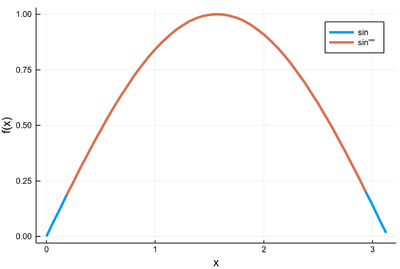
Study the derivatives to various orders of various functions. Replicate our previous analysis of the convergence and error of the first derivative as a function of the step size to higher orders.
We conclude with a fairly recent development that addresses precisely this problem, by turning to the complex plane. This applies only to so-called analytic functions but many of interest, especially in Physics, are, and to first-order derivatives but this is also the most common case and the gain in stability might make it worth to iterate this scheme instead of finite-difference higher order versions. The idea consists in taking the derivative of our otherwise real-valued function in the complex plane
$$f(x+ih)=f(x)+ihf'(x)-h^2{f''(x)\over2}+o(h^3)$$
so that our real derivative can be taken from the imaginary part as:
$$f'(x)=\operatorname{Im}\left({f(x+ih)\over h}\right)$$
that is to say, without a difference in the numerator. This is easily implemented in julia where a complex number $a+ib$ is written as complex(a,b) and the imaginary part from the imag() function, so that, e.g., a calculation of the error of our derivative of the sine in this way is obtained simply as:
julia> errcomplex=[mean(abs.([imag(sin(4pi*complex(x,δx)))/δx for x∈0:δx:1/16]
-[4pi*cos(4pi*x) for x in 0:δx:1/16])) for δx∈[2.0^-k for k∈4:31]]
28-element Array{Float64,1}:
 1.1372444664428887
 0.2854458844476824
 0.0718928022289436
 0.018064965628440573
 0.004529336363265703
 0.001134073879331725
 0.00028374242197300577
 7.09640059033831e-5
 1.7744576972572656e-5
 4.436592771446413e-6
 1.1092043576593092e-6
 2.77308116098488e-7
 6.932790813580023e-8
 1.7332086522437653e-8
 4.333035759267661e-9
 1.0832614533040955e-9
 2.708143764052942e-10
 6.770402313358929e-11
 1.692520694963255e-11
 4.231699645660417e-12
 1.0571258933920445e-12
 2.6388122953029493e-13
 6.716942649931662e-14
 1.5992600377570288e-14
 3.1984917211520782e-15
 1.5993687280109699e-15
 0.0
 0.0
The result becomes exact to within machine precision, and to visualize it in log-scale we substitute the exact zeros by the machine epsilon:
errcomplex[errcomplex.==0] .= eps()
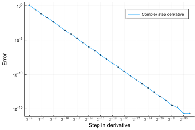
in which case one can see that the slope of the method is slow ($h^2$ only) but it does not suffer from numerical errors and thus can ultimately reach machine precision and stay pinned there:
plot(errcomplex, yscale=:log10, label="Complex step derivative");
scatter!(errcomplex, yscale=:log10, m=2, mc=palette(:default)[1], label="")
plot!(xticks = (1:2:30, ["\$2^{-$(k)}\$" for k∈4:30][1:2:end]), dpi=360,
      xformatter = :latex, xlabel = "Step in derivative", ylabel="Error")
