Crash Course in Scientific Computing
XIII. Root Finding
We have seen in the previous lecture as one of the earliest algorithm ever devised the one to compute the square root of 2. Looked at in a more general fashion, what this algorithm achieves is the particular case of a central problem of Mathematics: solving an equation. Namely, in this case:
$$f(x)=0\tag{1}$$
where $f(x)=x^2-2$. Nowadays, by completion of the square, we would solve Eq. (1) by writing it as $(x-\sqrt{2})(x+\sqrt{2})=0$ but this does not, actually, give us the numerical value. A computer would do this with a so-called root-finding algorithm. The simplest one is just a brute force approach where we compute all the values on a finite grid and take the closest one to the sought result. We can build the algorithm by steps:
# define a grid of trial points
δx=0.1;
lx=0:δx:2;

# Evaluate the function on this grid:
julia> (x->x^2-2).(lx)
21-element Array{Float64,1}:
 -2.0
 -1.99
 -1.96
 -1.91
 -1.8399999999999999
 -1.75
 -1.6400000000000001
 -1.51
 -1.3599999999999999
 -1.19
 -1.0
 -0.7899999999999998
 -0.56
 -0.30999999999999983
 -0.04000000000000026
  0.25
  0.5600000000000005
  0.8899999999999997
  1.2400000000000002
  1.6099999999999999
  2.0

# take the positive values:
abs.((x->x^2-2).(lx));

# find the smallest number (i.e., closest to zero):
julia> findmin(abs.((x->x^2-2).(lx)))
(0.04000000000000026, 15)
The smallest number is 0.04000000000000026, which is not very close to zero (only to within the first two digits), but that is not surprising given the coarse grid of points we took. This is obtained at the 15th index, so our approximate solution is:
julia> lx[findmin(abs.((x->x^2-2).(lx)))[2]]
1.4
which is not too bad for a wild guess:
julia> 1.4*1.4
1.9599999999999997

julia> 1.5*1.5
2.25
We can embed this "algorithm" into a (poor man's) root-find function:
# find x such that f(x)=0 in [a, b] with accuracy δx
function myfindroot(f, a, b, δx)
    lx=a:δx:b;
    lx[findmin(abs.((x->x^2-2).(lx)))[2]]
end
in which case we can, painfully, try to improve our accuracy. We know that the root was between the 15th and 16th element of our grid, so we can focus our search there:
julia> for k=2:10
        @time println(myfindroot(x->x^2-2, lx[15], lx[16], 10.0^-k))
       end
1.41
  0.000031 seconds (17 allocations: 544 bytes)
1.414
  0.000016 seconds (17 allocations: 1.234 KiB)
1.4142
  0.000021 seconds (17 allocations: 8.359 KiB)
1.41421
  0.000068 seconds (18 allocations: 78.625 KiB)
1.414214
  0.000772 seconds (18 allocations: 781.750 KiB)
1.4142136
  0.008025 seconds (18 allocations: 7.630 MiB)
1.4142135599999999
  0.153763 seconds (18 allocations: 76.294 MiB, 47.71% gc time)
1.4142135619999998
  0.839739 seconds (18 allocations: 762.940 MiB, 5.92% gc time)
Killed
That seems to work but the time, and eventually the resources, required crashed the machine. The problem is of course the number of points that we compute each time:
julia> length(2:10.0^-10:10)
80000000001
That's 80 billions, which is an overkill, when we only need to know the functions on the points close to root itself, not the whole range that extends far from it. The above implementation is an example of a working but inefficient, brute-force method that should be avoided. An algorithm should strive to optimize times and resources, and both if possible. A considerable improvement would be to return the interval surrounding the root for sure and focus our search there. This can be done by returning not our best estimates of the zero but its surrounding values, so that we can enclose both the root (and our best estimate of it):
function myfindroot(f, a, b, δx)
    lx=a:δx:b;
    x0=findmin(abs.(f.(lx)))[2]
    [lx[x0-1], lx[x0+1]]
end
Now this is immediate (a @time would show 0.000017 seconds (13 allocations: 656 bytes) for all entries!) and quickly converges to the result within machine precision:
julia> xmin=0; xmax=2;
       for k=1:16
           global xmin, xmax = myfindroot(x->x^2-2, xmin, xmax, 10.0^-k)
           println("$((xmin+xmax)/2)\t\t\t$(((xmin+xmax)/2)-sqrt(2))")
       end
1.4                     -0.014213562373095234
1.41                    -0.004213562373095225
1.4140000000000001      -0.0002135623730949998
1.4142                  -1.3562373095243885e-5
1.41421                 -3.5623730951783728e-6
1.4142139999999999      4.376269047146053e-7
1.4142136               3.762690492514764e-8
1.4142135599999999      -2.3730952758427293e-9
1.414213562             -3.730951103619873e-10
1.4142135624            2.690492273416112e-11
1.41421356237           -3.0950797480500114e-12
1.4142135623729999      -9.525713551283843e-14
1.4142135623731         4.884981308350689e-15
1.41421356237309        -5.10702591327572e-15
1.414213562373095       -2.220446049250313e-16
1.414213562373095       -2.220446049250313e-16
Compare to:
julia> sqrt(2)
1.4142135623730951
The error is that our method gives 1.4142135623730950 (last 0 added explictely) while the computer machine has 1.4142135623730951 so the difference is the last floating-point digit, which is eps() or -2.220446049250313e-16. Note that to within 22 decimals, the actual value is 1.4142135623730950488 so our result turns out to be in fact more accurate! While this is true in absolute precision, this doesn't matter in machine precision:
julia> 2-1.4142135623730951^2
-4.440892098500626e-16

julia> 2-1.4142135623730950^2
4.440892098500626e-16
Does it mean that we have completed our task of root-finding? This is, for instance, the seventh-root of three:
julia> xmin, xmax = 0, 2
for k=1:16
    global xmin, xmax = myfindroot(x->x^7-3, xmin, xmax, 10.0^-k)
end

julia> (xmin+xmax)/2
1.169930812758687

julia> (ans^7)
3.000000000000001
In fact, even this modest improvement, that spares us the computation of billions of useless points, is still very far from optimum, as we still compute the same number of points in each iterated loop, namely, that of our initial grid (since we divide the step by ten and apply it to one interval). So we, technically, still overcompute over a number of points that are not needed. Fixing this is not very complicated. Basically, we would just need to start with a minimal grid, which with our trick of surrounding the best guess, means three. In fact, one need only two points. That gives rise to the so-called bisection method which relies, for a continuous function, on the fact that on both sides of a "root", or "zero" (these are synonyms for "solution") of the equation, it has to change sign (assuming it is, of course, continuous). Therefore, one can halve the current interval in half and look for which one maintains this property: that is the one that contains the root. It could be that both feature this property, in which case one has at least three roots. A typical difficulty in finding roots is to finding all of them, in which case it helps considerably if we know how many of them we are looking for. On the other hand, we know the result we are looking for (zero), so we can keep looking until we reach the lowest possible accuracy, which is not compulsorily the machine epsilon. This is a possible julia implementation, where we stop if the algorithm didn't converge after some number of iterations (100 by default):
function bisection(f, a, b, maxit=100)
    c=(a+b)/2
    it=0
    while abs(f(c))>=eps() && it<maxit
        println("a=$(a)\t\t c=$(c)\t\t b=$(b)")
        println("f(a)=$(f(a))\t f(c)=$(f(c))\t f(b)=$(f(b))\n")
        if f(a)*f(c)<0
            b=c;
        else
            a=c;
        end
        c=(a+b)/2
        it+=1;
    end
    println("Result is $(c) obtained in $(it==100 ? "∞" : it) iterations with error $(f(c)-eps()/eps())ϵ.")
Our computation of $\sqrt{2}$ is such a case that needs fail-safe interruption as the result is larger than the machine epsilon:
julia> bisection(x->x^2-2,0,2)
a=0              c=1.0           b=2
f(a)=-2  f(c)=-1.0       f(b)=2

a=1.0            c=1.5           b=2
f(a)=-1.0        f(c)=0.25       f(b)=2

a=1.0            c=1.25          b=1.5
f(a)=-1.0        f(c)=-0.4375    f(b)=0.25

a=1.25           c=1.375                 b=1.5
f(a)=-0.4375     f(c)=-0.109375  f(b)=0.25

a=1.375          c=1.4375                b=1.5
f(a)=-0.109375   f(c)=0.06640625         f(b)=0.25

a=1.375          c=1.40625               b=1.4375
f(a)=-0.109375   f(c)=-0.0224609375      f(b)=0.06640625

a=1.40625                c=1.421875              b=1.4375
f(a)=-0.0224609375       f(c)=0.021728515625     f(b)=0.06640625

a=1.40625                c=1.4140625             b=1.421875
f(a)=-0.0224609375       f(c)=-0.00042724609375  f(b)=0.021728515625

a=1.4140625              c=1.41796875            b=1.421875
f(a)=-0.00042724609375   f(c)=0.0106353759765625         f(b)=0.021728515625

... skipped output ...

a=1.414213562373095              c=1.414213562373095             b=1.4142135623730951
f(a)=-4.440892098500626e-16      f(c)=-4.440892098500626e-16     f(b)=4.440892098500626e-16

a=1.414213562373095              c=1.414213562373095             b=1.4142135623730951
f(a)=-4.440892098500626e-16      f(c)=-4.440892098500626e-16     f(b)=4.440892098500626e-16

Result is 1.414213562373095 obtained in ∞ iterations with error -1.0000000000000004ϵ.
A simple but good improvement is the Newton–Raphson method (Newton used it for the particular case of polynomials; Raphson extended it to arbitrary functions). The idea is to start with a blind guess $x_0$ around the solution and replace the real function $f(x)$ by a linear approximation with the same slope at $x_0$, i.e., $h(x)=f'(x_0)x+\beta$ with $\beta$ such that $h(x_0)=f(x_0)$ which yields
$$h(x)=f'(x_0)[x-x_0]+f(x_0)$$
Now a better guess for the zero is found by solving $h(x)=0$ which has solution $x=x_0-(f(x_0)/f'(x_0))$. Of course the procedure can be iterated so the algorithm gives us the always better approximations:
$$x_{n+1}=x_n-{f(x_n)\over f'(x_n)}\,.$$
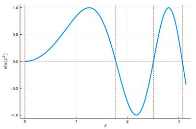
Let us find the zeros of $f(x)=\sin(x^2)$ between 0 and $\pi$. It's good to know beforehand the sort of results we expect (we added vertical lines by eye):
psin2=plot(x->sin(x^2), 0, π,
ylabel=L"\sin(x^2)",xlabel=L"x",lw=3,
legend=false)
vline!([0, 1.77, 2.51, 3.07], line = (:red, :dash, 1))
hline!([0], line = (:black, :dot, .75))

The formula gives us:
$$x_{n+1}=x_n-{\sin x_n^2\over 2x_n\cos x_n^2}$$
We can write a function that takes $f/f'$ as an input (that we have to compute ourselves) that computes such iterations until the procedure differs by less than some $\epsilon$:
function NewtonRaphson(f, x0)
    ϵ=10^-16
    x1=x0+10ϵ
    while abs(x1-x0)>ϵ
        x0=x1
        x1=x0-f(x0)
    end
    x1
end
This provides the values found in the $[0,\pi]$ interval:
lsols=[NewtonRaphson(x->sin(x^2)/(2*x*cos(x^2)), x) for x in 0:.01:π]
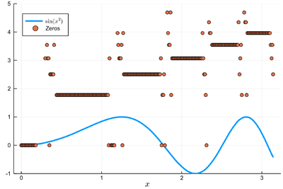
We can plot the solutions together with where was the starting point:
psin2=plot(x->sin(x^2), 0, π,
label=L"\sin(x^2)",xlabel=L"x",
legend=:bottomleft)

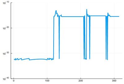
We found many, in particular some outside the $[0,\pi]$ range (this was the case when the tangent was sending us far away). We can check these are indeed all solutions:
plot(abs.(sin.(lsols.^2)), yscale=:log10, ylims=(10^-40,10^-10), legend=false)

To actually extract the values, we could use unique(), but this would return a lot of different values for the 0 zero, so we'd round this:
lsolss=sort(unique(round.(lsols,digits=10)))
These are the said solution in the sought range:
lsolss[findall(x-> 0<=x<=π, lsolss)]
5-element Array{Float64,1}:
 -0.0
  0.0
  1.7724538509
  2.5066282746
  3.0699801238
-0.0 and 0.0 are seen as different in julia, surely something that'll be fixed eventually. We have four solutions, as is clear from the initial graph.
There is a Roots package that has a function fzero() that achieves something similar:
fzero(x->sin(x^2), 2)
1.772453850905516