Crash Course in Scientific Computing

VI. Random Numbers

We now turn to another types of special numbers, which also have a special type of relationship with computers, namely, random numbers. That will allow us to play with things that computers are good at (e.g., with statistics). We'll need another package first:

import Pkg; Pkg.add("Distributions")

Once this is done (once for ever on a given machine), you can then be:

using Distributions

What is a random number? Something you can't predict, e.g.,

julia> rand()
0.663764152328755

julia> rand()
0.017345425057746944

julia> rand()
0.6186819567638984

although in these three cases, one can see that the numbers are between 0 and 1, so it is tempting to predict they'll maintain that pattern, and one can check they do. This is because even random numbers follow some rules, or law, or, more accurately, distribution. Namely, the distribution of random numbers is the mathematical functions that gives the probability that any given sampling will be found in a given range. The rand() distribution returns a random number uniformly (i.e., with same probability) distributed between, indeed, 0 and 1. To see that with our own eyes, let us generate ten thousands such random points and plot an histogram, which is a sort of empirical distribution, approaching the theoretical one that generates the numbers from a sampling of its output:

lst=[rand() for i=1:10^5]

and after

using Plots
histogram(lst)

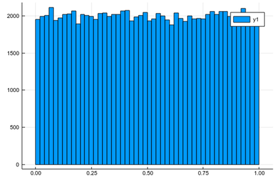
As expected. The fact that this is not a straight line but jumps from one window to the other is called "fluctuation". This is typical of random numbers. The more we have, the less they will fluctuate around their theoretical value. Now let us ask ourselves, what would be the distribution if we square each random number after drawing it? We can call $X$ the so-called random variable which returns a random number following a given distribution, here, uniform between 0 & 1, so we could write $X\to U([0,1])$. We are then asking, what is the distribution of $X^2$? Is it still uniform? One thing is for sure, is that since $0\le X\le 1$, then also $0\le X^2\le1$. Let us ask the computer what it finds:

lst=[rand()^2 for i=1:10^5]
histogram(lst)

and after

using Plots

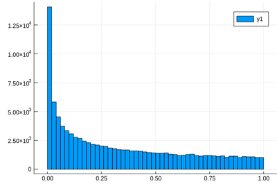
This has a clear structure which is not the straight line anymore. Not surprisingly, squared numbers are not uniform. Some people explain it as the square of a small number being smaller than the number itself, so will tend to pile up towards zero. But then shouldn't we expect numbers above 1 to clutter towards larger values? The random variable $2X$ is uniformly distributed over $[0,2]$, but $(2X)^2$ is clearly $4X^2$ and multiplying by 4 the $X^2$ random variable, which has the shape shown above, will not change its structure. More accurately, therefore, this is due to the concavity of the function, rather than its relation to the identity. We can get a better understanding by hunting the theoretical result, which the computer can help us to check, or give us clues, but we shouldn't rely on the computer alone to understand what is going on.

The exact result is obtained by differentiating the cumulative function, $f_{X^2}=dF_{X^2}/dx$, with $F_{X^2}(x)\equiv=\int_0^x f_{X^2}(y)\,dy$. This follows from the fundamental theorem of calculus. Now, since from the interpretation of $f_{X^2}$ as a density of probability, we have

$$F_{X^2}(x)=\mathbb{P}(X^2\le x)$$

where $\mathbb{P}(X^2\le x)$ is the probability for $X^2$ to be less than $x$, then we can compute $\mathbb{P}(X^2\le x)=\mathbb{P}(X\le\sqrt{x})=\sqrt{x}$, since the probability is uniform. Therefore:

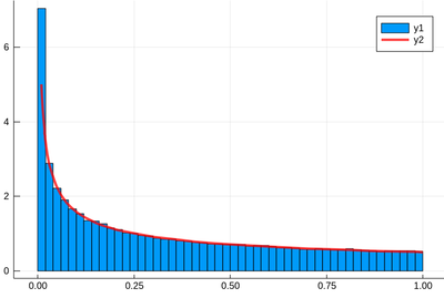
$$f_{X^2}(x)={1\over2\sqrt{x}}\,.$$

Let us check:

f(x)=1/(2*sqrt(x))
histogram(lst,norm=true)
plot!(f,.01,1, linewidth = 4, linecolor = :red, linealpha=0.75)

Remember that ! means to plot on the existing display and we've used the option norm=true to normalize the histogram, effectively turning it into a probability distribution. This seems to work indeed:

Let's have a look at the distribution of inverse random numbers, also sampled from a uniform distribution between 0 and 1. This time, the support is infinite (it is $[1,\infty[$). The theoretical distribution is $f_{1/X}=d\mathbb{P}_{1/X}/dx$ with $\mathbb{P}_{1/X}=\mathbb{P}(1/X\le x)=\mathbb{P}(X\ge 1/x)=1-1/x$ (being uniform again), so that $f_{1/X}(x)=1/x^2$.

This time we'll use a lot of points to make sure we get the exact result:

@time lst = [1/rand() for i=1:10^8]

The @time allows us to benchmark the time and memory resources involved. As you can see, on a 2020 machine, it's pretty fast (for a hundred million points!)

  0.427357 seconds (67.69 k allocations: 766.257 MiB, 0.65% gc time)

The result is also consequently very smooth:

@time histogram(lst,norm=true,bins=0:.01:10)

returning

4.644046 seconds (4.88 k allocations: 1.490 GiB, 1.74% gc time)

and, after also

f(x)=1/x^2
plot!(f,1,10,linewidth=4,linecolor=:red,linealpha=.75)

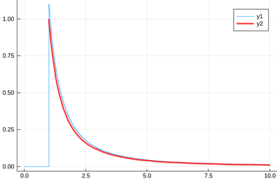
This is slightly off, clearly. The culprit is our empirical (i.e., computed) distribution function, which density should be 1 at $x=1$ and is more than that. The problem is the norm option of histogram, which normalizes to what is plotted (or retained). And we have points beyond that. It would work better if we'd plot more points but we wouldn't see much over a larger range. Instead, we can use the correct number to renormalize our theory plot. This is how many numbers we have:

sum(lst .< 10)

You can use this to check that we have the correct distribution (Solution).

and, although this is not needed, this is the list of the numbers we exclude:

lst[lst .> 100]

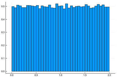
Let us look at other operations on random variable. You can easily convince yourself that rescaling a random variable $X$ by a constant $\alpha$ merely rescale the range of these numbers, or the support of the distribution, which needs to remain normalized though so in effect we are stretching the space. For instance $2X$ has its distribution function normalized to $1/2$:

histogram([2rand() for i=1:10^5], norm=true, legend=false)

How about, not $2X$, which is of course $X+X$, but $X+Y$ where both $X$ and $Y$ follow the same uniform distribution $U([0,1])$. Is that $2X$ again since $X$ and $Y$ are the same? Careful: the fact that $X$ and $Y$ follow the same distribution does not mean that they are equal, $X\neq Y$. Each time that we look at the variable, it takes a different value (it is random)

julia> X, Y = rand(), rand()
(0.023904897028309557, 0.8702240210821197)
 
julia> X==Y
false

The actual instances are different but surely the distribution would be the same and that of $2X$ (or $2Y$)? Let us find out:

histogram([rand()+rand() for i=1:10^5], norm=true, legend=false)

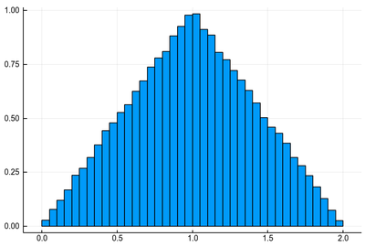
Clearly not uniform. In fact, it is an exact triangle! The phenomenon here is that while $X$ and $Y$ can take any value between 0 and 1 with the same probability, it is more likely for their sum to be close to their average. If that surprises you, do the same reasoning with two dices. What probability do you get to draw a 7 as compared to drawing a 2 or a 12? The exact distribution for $X+Y$ can be found by similar reasoning but with a continuous variable. It is easily done geometrically. More generally, in probability theory, one can show that the sum of two independent random variables follows the distribution given by the convolution of the distribution of the random variables, which also explains this triangular shape and allows to extend it to greater sums

$$\sum_{i=0}^n X_i\tag{1}$$

which give rise to the Irwin-Hall distributions:

Consider the sum of $k$ independent random variables $X_i$ uniformly distributed over $[0,1]$. Study numerically the distribution function of their sum, Eq. (1) and check that this is given by the Irwin-Hall formula:

$${f_{X}(x;n)={\frac {1}{2(n-1)!}}\sum _{k=0}^{n}(-1)^{k}{n \choose k}(x-k)^{n-1}\operatorname{sgn}(x-k)}\tag{2}$$

where

$${\operatorname {sgn}(x-k)\equiv{\begin{cases}-1&x<k\\0&x=k\\1&x>k.\end{cases}}}$$ (Answer)

Equation (2) is a funny composition of functions, namely, stiched piecewise polynomials (so-called splines). for instance, the case $n=3$ gives:

$${f_{X}(x)={\begin{cases}{\frac {1}{2}}x^{2}&0\leq x\leq 1\\{\frac {1}{2}}(-2x^{2}+6x-3)&1\leq x\leq 2\\{\frac {1}{2}}(x-3)^{2}&2\leq x\leq 3\end{cases}}}$$

which, regardless of its odd definition, has a very natural look especially as $n$ becomes larger. From the above exercise:

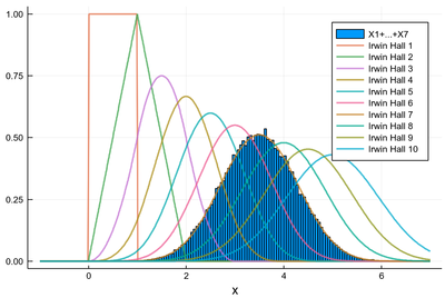
In the limit where $n\to\infty$, these distributions tend to some familiar function: the Gaussian. This is the result of the so-called central limit theorem that asserts that, not only uniform distributions, but any type of independent random variables, when summed in large numbers, tend to what is called a normal distribution, where the denomination of "normal" comes from its widespread occurrences and natural-looking character, making it the distribution one expects to find when things are "normal".

The normal distribution takes two parameters, the mean $\mu$ and the standard deviation $\sigma$. This is how we define such a distribution in julia (here with mean 1 and standard deviation 0.5):

julia> dist=Normal(1.0, .5)
Normal{Float64}(μ=1.0, σ=0.5)

We can now generate normally-distributed random numbers:

julia> rand(dist)
0.6696409682501712

julia> rand(dist)
0.6985762003105883

julia> rand(dist)
1.8506284482154651

In the laboratory, we would ask you to find the mean of a normally distributed random variable by using five points. Does it work?

julia> mean([rand(dist) for i=1:5])
0.6439917898168767

Ouch! We were expecting 1!

julia> dist.μ
1.0

So? Oh! We're doing statistics... things vary from one realization to the other:

julia> mean([rand(dist) for i=1:5])
0.5196060896076187

julia> mean([rand(dist) for i=1:5])
1.109368345414772

julia> mean([rand(dist) for i=1:5])
1.1134351116298737

julia> mean([rand(dist) for i=1:5])
1.235455527271116

julia> mean([rand(dist) for i=1:5])
1.2718188614651438

Of course, there are a lot of fluctuations... We had, after all a big standard deviation:

julia> dist.σ
0.5

So don't forget to plot error bars in your graphs!

An important theme of statistics is to study the statistical behaviour of statistical quantities, e.g., how does the mean itself fluctuate? Let's find out:

sample=[rand(dist) for i=1:10^5];
histogram(sample, norm=true, label="Normally distributed numbers")
samplemean=[mean([rand(dist) for i=1:5]) for j=1:10^5];
histogram!(samplemean, norm=true, label="Distribution of their mean")

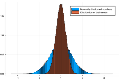
The different bin-sizes is due to the different support for both cases, this could be enforced with the bins option.

So the mean looks like it's also fluctuating normally, with the same mean but with a different (smaller) standard deviation. In fact, one can show that the standard deviation $\sigma_M$ of the mean of $N$ numbers relates to the standard deviation $\sigma$ of the numbers themselves (if normally distributed) as follows:

$$\sigma_M={\sigma\over\sqrt{N}}$$

What is the distribution of the standard deviation $\sigma=\sqrt{\operatorname{var}(X)}$? This cannot be normal since it must be a positive number, the square root of the variance $\operatorname{var}$ which is itself, for $n$ numbers, defined as:

$$\operatorname{var}(\{x_1,\cdots,x_n\})={1\over n}\sum{i=1}^n(x_i-\langle x\rangle)^2\tag{3}$$

What is it then? Let's ask the computer before we ask the theory:

histogram([std([rand(dist) for i=1:3], corrected=false) for j=1:10^5], norm=true, label="Distribution of standard deviation")

The option corrected=false is to ensure that std computes the square root of the variance as defined by Eq. (3), since there are various definitions.

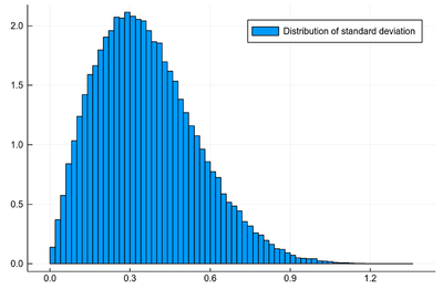
Clearly the standard deviation is not normally distributed. Remember that the standard deviation of the initial distribution was $\sigma=1/2$. Can we get access to that?

julia> mean([std([rand(dist) for i=1:3], corrected=false) for j=1:10^5])
0.36240524388003825
 
julia> mean([std([rand(dist) for i=1:3], corrected=false) for j=1:10^5])
0.36003512501085244
 
julia> mean([std([rand(dist) for i=1:3], corrected=false) for j=1:10^5])
0.36149996456935973

Not really... Theory tells us that the distribution of the standard deviation is a complex function involving the $\Gamma$ function, whose mean is related to the standard deviation of the starting distribution by a factor of $\sqrt{2/N}\Gamma(N/2)/\Gamma((N-1)/2)$ where $N$ is the number of points used to estimate the standard deviation. And indeed:

julia> using SpecialFunctions
julia> bN=sqrt(2/N)*gamma(N/2)/gamma((N-1)/2)
0.7236012545582677
 
julia> mean([std([rand(dist) for i=1:3], corrected=false) for j=1:10^5])/bN
0.5011040338393551

which is the good result ($\sigma=1/2$).

Let us now explore numerically a very interesting (and important) phenomenon. For that, we'll need the Cauchy function from the above-loaded "Distributions" package. This is a histogram of $10^5$ Cauchy-distributed points:

histogram(rand(Cauchy(),10^5))

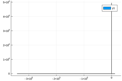
Here the binning is mandatory:

histogram(rand(Cauchy(),10^5),bins=-10:.5:10,norm=true)

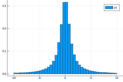
Above, we have dealt with continuous distributions ...

discrete distributions:

The most important one is the Poisson distribution. It takes one parameter

julia> P=Poisson(3)
Poisson{Float64}(λ=3.0)

It gives the number of events which can happen in the unit time:

julia> rand(P)
5
 
julia> rand(P)
1
 
julia> rand(P)
1
 
julia> rand(P)
1
 
julia> rand(P)
2
 
julia> rand(P)
3
 
julia> rand(P)
0

julia> λ=3
 
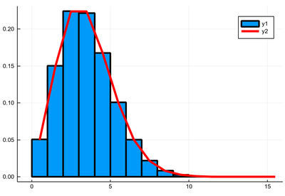
julia> histogram([rand(P) for i=1:10^5],norm=true,bins=0:15)
 
julia> plot!(collect(0:15).+.5, [λ^k*exp(-λ)/factorial(k) for k=0:15], lw=4, lc=:red)

Variance is equal to the mean:

julia> var([rand(P) for i=1:10^5])
3.0059645571455715
 
julia> mean([rand(P) for i=1:10^5])
2.98864

---

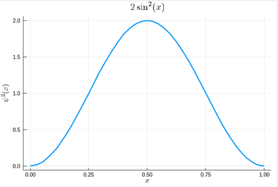
Let us conclude with a brief look at how to generate random numbers on our own, that is, following any given probability distribution (a positive, normalized function). For instance, let us say we want to simulate the ground state of a particle in a box, with probability distribution over $[0,1]$ given by:

$$\psi^2(x)=2\sin^2(\pi x)$$

We remind that one can use unicode characters (by entering \psi+TAB) to call our density of probability ψ2, which in quantum mechanics is given by the modulus square of the probability amplitude (in 1D the wavefunction can always be taken real so we do not need worry about the modulus):

ψ2(x)=2*sin(pi*x)^2

That's our density of probability:

using LaTeXStrings
default(; w=3)
plot(ψ2,0,1, title=L"2\sin^2(x)", xlabel=L"x", ylabel=L"\psi^2(x)",dpi=150,legend=false)

where we decorated the plot with a lot of options, but the width which we gave as a default attribute, not to do it in the future (and since we like thick lines).

We will compute $\int_0^1\psi^2(x)\,dx$ by computing Riemann sums, i.e., as a sum of parallelograms defined in a partition of the support of the function (here $[0,1]$) cut into $n$ intervals. Calling $f$ the function to integrate, this is defined as:

$$R_n=\sum_{i=1}^{n}f(x_i)\delta(i)$$

a, b = 0, 1; # boundaries
lx=range(a, stop=b, length=11) # list of x intervals
δ=diff(lx) # widths of intervals
lxi=lx[1:end-1] # x_i points of parallelograms

We can now check the normalization:

sum([ψ2(lxi[i])*δ[i] for i=1:length(lxi)])

1.0

The cumulative is obtained as:

Ψ=[sum([ψ2(lxi[i])*δ[i] for i=1:j]) for j=1:length(lxi)]

This is the result for 100 intervals (length=101 above):

plot(lxi, Ψ, legend=false, title="Cumulative")

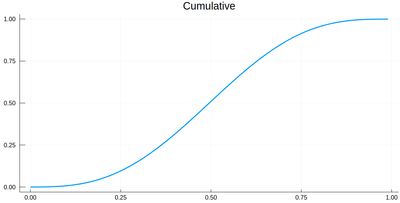
Now the generation of a random number following the initial distribution works as follows. We select randomly (uniformly) a number on the $y$-axis of the cumulative and find the corresponding $x$ such that $F(x)=y$. Those $x$ are $f$ distributed.

This can be simply achieved as follows (later we'll see a more sophisticated way):

yr=rand()
fx=lx[[findmin(abs.(Ψ.-rand()))[2] for i=1:10]]

Here are some positions where our ground state collapsed:

10-element Array{Float64,1}:
 0.55
 0.96
 0.24
 0.5 
 0.58
 0.16
 0.67
 0.74
 0.08
 0.46

histogram(lx[[findmin(abs.(Ψ.-rand()))[2] for i=1:10^7]], bins=0:.01:1,norm=true)

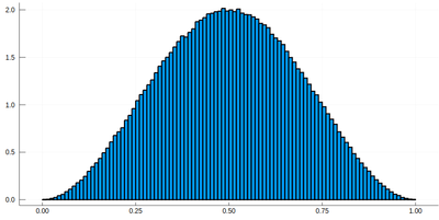
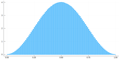
Note that the binning cannot be less than the $\delta$ step, otherwise we will get "holes" (and also the wrong normalization):

histogram(lx[[findmin(abs.(Ψ.-rand()))[2] for i=1:10^7]], bins=0:δ[1]/2:1,norm=true)

We would typically want to embed our results together in a function of our own:

function myRiemann(f, n)
    a, b = 0, 1; # boundaries
    lx=range(a, stop=b, length=n) # list of x intervals
    δ=diff(lx); # widths of intervals
    lxi=lx[1:end-1]; # x_i points of parallelograms
    sum([f(lxi[i])*δ[i] for i=1:length(lxi)])
end

Then we can try:

myRiemann(g, 10^3)

The result is fairly close to the exact $e-1\approx1.718281828459045$:

1.717421971020861

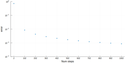
However we'll find that our method is fairly limited:

scatter([abs(myRiemann(g, i)-(exp(1)-1)) for i=2:100:1002], 
  ylims=(10^-4,1), yscale=:log10, xticks=(1:11, 2:100:1002), 
  xlabel="Num steps", ylabel="error")

It is the purpose of numerical methods to learn how to use algorithms that are efficient, in the sense that they are accurate, fast and resource-effective.

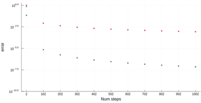
It is easy to be brutal and terribly inefficient with a computer. In fact a fairly trivial enhancement of our method leads to considerable improvement:

function myRiemann(f, n, method="mid")
    a, b = 0, 1; # boundaries
    lx=range(a, stop=b, length=n) # list of x intervals
    δ=diff(lx); # widths of intervals
    if method == "left"
        lxi=lx[1:end-1]; # x_i points of parallelograms
    elseif method == "right"
        lxi=lx[2:end];
    else
        lxi=(lx[1:end-1]+lx[2:end])/2;
    end
    sum([f(lxi[i])*δ[i] for i=1:length(lxi)])
end

Of course, other people already wrote such functions, that are available through packages. For numerical integration of 1D functions, one can use QuadGK which is based on the so-called Gauss–Kronrod quadrature formula, which basically figures out how to best choose the points $x_i$ and how to weight them:

using QuadGK
@time quadgk(g, 0, 1)

Unlike our naive implementation, the result is pretty accurate:

  0.000034 seconds (9 allocations: 304 bytes)
(1.718281828459045, 0.0)

That's the best we can achieve (with mid-points and a hundred-million intervals!)

@time myRiemann(g, 10^8)

    9.762264 seconds (500.00 M allocations: 8.941 GiB, 11.01% gc time)
1.7182818284590453

It differs from the exact result only in the last digit, but took about 10s & 9GiB of memory.

Links

• Related discussion from my Computación I lectures at the Universidad Autónoma de Madrid.