Crash Course in Scientific Computing

XIII. Integrals

Let us conclude with a brief look at how to generate random numbers on our own, that is, following any given probability distribution (a positive, normalized function). For instance, let us say we want to simulate the ground state of a particle in a box, with probability distribution over $[0,1]$ given by:

$$\psi^2(x)=2\sin^2(\pi x)$$

We remind that one can use unicode characters (by entering \psi+TAB) to call our density of probability ψ2, which in quantum mechanics is given by the modulus square of the probability amplitude (in 1D the wavefunction can always be taken real so we do not need worry about the modulus):

ψ2(x)=2*sin(pi*x)^2

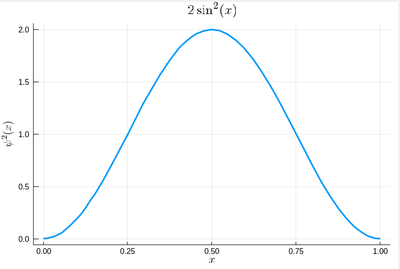
That's our density of probability:

using LaTeXStrings
default(; w=3)
plot(ψ2,0,1, title=L"2\sin^2(x)", xlabel=L"x", ylabel=L"\psi^2(x)",dpi=150,legend=false)

where we decorated the plot with a lot of options, but the width which we gave as a default attribute, not to do it in the future (and since we like thick lines).

We will compute $\int_0^1\psi^2(x)\,dx$ by computing Riemann sums, i.e., as a sum of parallelograms defined in a partition of the support of the function (here $[0,1]$) cut into $n$ intervals. Calling $f$ the function to integrate, this is defined as:

$$R_n=\sum_{i=1}^{n}f(x_i)\delta(i)$$

a, b = 0, 1; # boundaries
lx=range(a, stop=b, length=11) # list of x intervals
δ=diff(lx) # widths of intervals
lxi=lx[1:end-1] # x_i points of parallelograms

We can now check the normalization:

sum([ψ2(lxi[i])*δ[i] for i=1:length(lxi)])

1.0

The cumulative is obtained as:

Ψ=[sum([ψ2(lxi[i])*δ[i] for i=1:j]) for j=1:length(lxi)]

This is the result for 100 intervals (length=101 above):

plot(lxi, Ψ, legend=false, title="Cumulative")

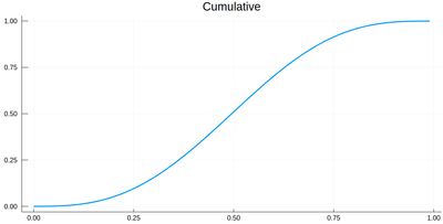
Now the generation of a random number following the initial distribution works as follows. We select randomly (uniformly) a number on the $y$-axis of the cumulative and find the corresponding $x$ such that $F(x)=y$. Those $x$ are $f$ distributed.

This can be simply achieved as follows (later we'll see a more sophisticated way):

yr=rand()
fx=lx[[findmin(abs.(Ψ.-rand()))[2] for i=1:10]]

Here are some positions where our ground state collapsed:

10-element Array{Float64,1}:
 0.55
 0.96
 0.24
 0.5 
 0.58
 0.16
 0.67
 0.74
 0.08
 0.46

histogram(lx[[findmin(abs.(Ψ.-rand()))[2] for i=1:10^7]], bins=0:.01:1,norm=true)

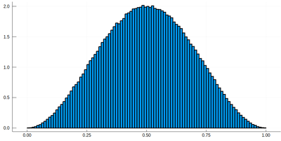
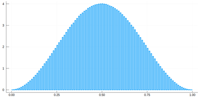
Note that the binning cannot be less than the $\delta$ step, otherwise we will get "holes" (and also the wrong normalization):

histogram(lx[[findmin(abs.(Ψ.-rand()))[2] for i=1:10^7]], bins=0:δ[1]/2:1,norm=true)

We would typically want to embed our results together in a function of our own:

function myRiemann(f, n)
    a, b = 0, 1; # boundaries
    lx=range(a, stop=b, length=n) # list of x intervals
    δ=diff(lx); # widths of intervals
    lxi=lx[1:end-1]; # x_i points of parallelograms
    sum([f(lxi[i])*δ[i] for i=1:length(lxi)])
end

Then we can try:

myRiemann(g, 10^3)

The result is fairly close to the exact $e-1\approx1.718281828459045$:

1.717421971020861

However we'll find that our method is fairly limited:

scatter([abs(myRiemann(g, i)-(exp(1)-1)) for i=2:100:1002], 
  ylims=(10^-4,1), yscale=:log10, xticks=(1:11, 2:100:1002), 
  xlabel="Num steps", ylabel="error")

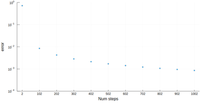
It is the purpose of numerical methods to learn how to use algorithms that are efficient, in the sense that they are accurate, fast and resource-effective.

It is easy to be brutal and terribly inefficient with a computer. In fact a fairly trivial enhancement of our method leads to considerable improvement:

function myRiemann(f, n, method="mid")
    a, b = 0, 1; # boundaries
    lx=range(a, stop=b, length=n) # list of x intervals
    δ=diff(lx); # widths of intervals
    if method == "left"
        lxi=lx[1:end-1]; # x_i points of parallelograms
    elseif method == "right"
        lxi=lx[2:end];
    else
        lxi=(lx[1:end-1]+lx[2:end])/2;
    end
    sum([f(lxi[i])*δ[i] for i=1:length(lxi)])
end

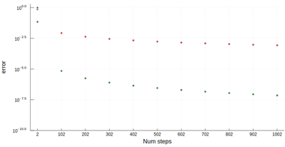
Of course, other people already wrote such functions, that are available through packages. For numerical integration of 1D functions, one can use QuadGK which is based on the so-called Gauss–Kronrod quadrature formula, which basically figures out how to best choose the points $x_i$ and how to weight them:

using QuadGK
@time quadgk(g, 0, 1)

Unlike our naive implementation, the result is pretty accurate:

  0.000034 seconds (9 allocations: 304 bytes)
(1.718281828459045, 0.0)

That's the best we can achieve (with mid-points and a hundred-million intervals!)

@time myRiemann(g, 10^8)

    9.762264 seconds (500.00 M allocations: 8.941 GiB, 11.01% gc time)
1.7182818284590453

It differs from the exact result only in the last digit, but took about 10s & 9GiB of memory.