Overlay of a Mathematica plot with an image

⇠ Back to Blog:Science

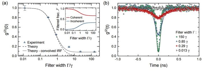
One often wants to compare a printed graph with one's own Mathematical curve. When the curve is fixed, I use Inkscape to do that, with opacity of either one of the images. That's the simplest. If the curve is varying, however, one can use Mathematica's Manipulate to do something similar, on the go. Here's an example that comes from a nice paper from Sheffield & Manchester on the Photon Statistics of Filtered Resonance Fluorescence, by Catherine Phillips et al. There, among other things, they checked the loss of antibunching in resonance fluorescence that we theorized in a series of papers. This is their Fig. 2:

Now in Ref. , we have a theoretical formula (Eq. (19b)) for what should be the theory curve on the left. In tidied-up notations, this is:

$$g^{(2)}(\tau=0)=\frac{\digamma_{11}\left(\gamma_\sigma ^2+4 \Omega ^2\right) \left(\digamma_{11}\digamma_{12}+8 \Omega ^2\right) \left(48 \Gamma ^2 \Omega ^4 \digamma_{21}+4 \Gamma \Omega ^2 \digamma_{31} \left(17 \Gamma ^3+29 \Gamma ^2 \gamma_\sigma +18 \Gamma \gamma_\sigma ^2+4 \gamma_\sigma ^3\right) +\digamma_{11}\digamma_{21}^2\digamma_{31}^2 \digamma_{12}\digamma_{32}\right)} {\digamma_{21}\digamma_{31}\left(\digamma_{11}\digamma_{21}+4 \Omega ^2\right) \left(\digamma_{31}\digamma_{32}+8 \Omega ^2\right) \left(\digamma_{12}\digamma_{11}^2 +4 \Gamma \Omega ^2\right)^2}$$

where we defined $\digamma_{kl}\equiv k\Gamma+l\gamma_\sigma$, for $\gamma_\sigma$ the radiative decay rate of the two-level system, $\Gamma$ the filter's bandwidth and $\Omega$ the driving strength. We also studied the same problem from the experimental perspective with Lukas Hanschke from the TUM et al. and find similar things (with a better agreement), as shown in Ref. , where the above equation appears in this very form as Eq. (20). The point is, is this "similar" exactly the same? Is our analytical expression a perfect match to their theory curve? Our colleagues do not give a closed-form expression for this result and we can only surmise they got it numerically. How do the two compare? We have a better agreement with the TUM data so although in print it should be the same, maybe it's not. Then comes the problem of comparing a printed graph with your own Mathematical curve.

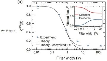
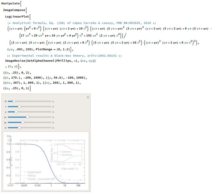
This is how to do it in Mathematica, combining ImageCompose, ImageResize & SetAlphaChannel:

The image is screenshot and pasted directly into the notebook & defined as something (here, Phillips, after the first author) and the following code that includes x and y to position horizontalwise & verticalwise the image, and sx, sy to scale it, so as to align it with the Mathematica plot, and α to change the transparency (opacity):

In code (you can copy/paste this in a notebook but you'll need to define the image):

Manipulate[
 ImageCompose[
  LogLinearPlot[
   (* Analytical formula, Eq. (19b) of López Carreño & Laussy, PRB 94:
   063825, 2016 *)
   ((\[Gamma]a + \[Gamma]\[Sigma]) (\[Gamma]\
\[Sigma]^2 + 
        8 \[CapitalOmega]^2) ((\[Gamma]a + \[Gamma]\[Sigma]) \
(\[Gamma]a + 2 \[Gamma]\[Sigma]) + 
        16 \[CapitalOmega]^2) ((\[Gamma]a + \[Gamma]\[Sigma]) (2 \
\[Gamma]a + \[Gamma]\[Sigma])^2 (3 \[Gamma]a + \[Gamma]\[Sigma])^2 (\
\[Gamma]a + 2 \[Gamma]\[Sigma]) (3 \[Gamma]a + 2 \[Gamma]\[Sigma]) + 
        8 \[Gamma]a (3 \[Gamma]a + \[Gamma]\[Sigma]) (17 \[Gamma]a^3 \
+ 29 \[Gamma]a^2 \[Gamma]\[Sigma] + 18 \[Gamma]a \[Gamma]\[Sigma]^2 + 
           4 \[Gamma]\[Sigma]^3) \[CapitalOmega]^2 + 
        192 \[Gamma]a^2 (2 \[Gamma]a + \[Gamma]\[Sigma]) \
\[CapitalOmega]^4))/((2 \[Gamma]a + \[Gamma]\[Sigma]) (3 \[Gamma]a + \
\[Gamma]\[Sigma]) ((\[Gamma]a + \[Gamma]\[Sigma]) (2 \[Gamma]a + \
\[Gamma]\[Sigma]) + 
        8 \[CapitalOmega]^2) ((3 \[Gamma]a + \[Gamma]\[Sigma]) (3 \
\[Gamma]a + 2 \[Gamma]\[Sigma]) + 
        16 \[CapitalOmega]^2) ((\[Gamma]a + \[Gamma]\[Sigma])^2 (\
\[Gamma]a + 2 \[Gamma]\[Sigma]) + 8 \[Gamma]a \[CapitalOmega]^2)^2),
   {\[Gamma]a, .001, 250}, PlotRange -> {0, 1.2}],
    (* Experimental results & black-box theory, arXiv:2002.08192 *)
  
  ImageResize[SetAlphaChannel[Phillips, \[Alpha]], {sx, sy}]
  , {x, y}],
 {{\[CapitalOmega], .25}, 0, 2}, {{x, 179.}, -100, 
  1000}, {{y, 94.8}, -100, 1000}, {{sx, 367}, 1, 800, 1}, {{sy, 268}, 
  1, 800, 1}, {{\[Alpha], .25}, 0, 1}]

For those who are interested in the Physics: it's a perfect match (at the driving the Authors give, with different conventions, so all is correct). Therefore, for some reason, the data from TUM is simply "better" (we do not need to further process the data with deconvolution which we furthermore think are not exact for two-photon observables, and even so, they have one point badly off the curve). In both cases, however, these are great results that should give a new twist to coherently driven quantum emitters, and Phillips et al. also make very good points at higher driving.

— Fabrice • 11:42, 18 May 2020