

Next: Second order correlation function Up: Theoretical Background Previous: The manifold approach Contents
The Quantum Regression Formula
The quantum regression formula (QRF) found by Lax (1963),
(1967) provides a method to compute any two-time
correlator from a master equation of the form
![]() [Eq. (2.71)] (for system interacting
with Markovian reservoirs). As demonstrated in the book by
Carmichael (2002), once one has found a set of
operators
[Eq. (2.71)] (for system interacting
with Markovian reservoirs). As demonstrated in the book by
Carmichael (2002), once one has found a set of
operators
![]() that satisfy
that satisfy
for the general operator
The Hilbert space of correlators is separated in manifolds,
just as the Hilbert space of states is separated in manifolds of
excitation. The order ![]() of a manifold is the minimum number of
particles that should be in the system (regardless of the regression
matrix) so that the correlator is nonzero. Equivalently, it is the
minimum manifold of excitations that should be probed in the
dynamics. We will refer to the two-time and one-time correlator
manifolds as
of a manifold is the minimum number of
particles that should be in the system (regardless of the regression
matrix) so that the correlator is nonzero. Equivalently, it is the
minimum manifold of excitations that should be probed in the
dynamics. We will refer to the two-time and one-time correlator
manifolds as
![]() and
and
![]() ,
respectively.
,
respectively.
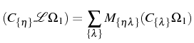
The first step is to find the set of operators that are needed to
compute the correlator of interest. For example, in the case of
bosons, in order to set the equations to obtain
![]() , we consider
, we consider
![]() . If this is
the only field involved in the dynamics, the most general set of
operators in normal order can be written as
. If this is
the only field involved in the dynamics, the most general set of
operators in normal order can be written as
![]() . For the simple problem of a thermal
bath, it is enough to consider only
. For the simple problem of a thermal
bath, it is enough to consider only ![]() . The only matrix element
is
. The only matrix element
is
![]() and the correlator can
be trivially integrated taking as the initial state the SS value
and the correlator can
be trivially integrated taking as the initial state the SS value
![]() :
:
![]() . The spectra is
again a Lorentzian
. The spectra is
again a Lorentzian
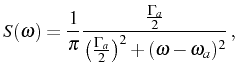
this time broadened by a renormalized bosonic decay rate:
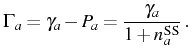
In this case, in order to have a physical SS (finite populations and correlations which decay with time), we know that the parameters
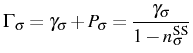
which is different from the decay rate in vacuum
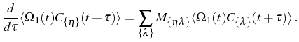
In more complicated systems, the correlator of interest will depend on
other correlators, giving rise to a set of coupled equations of the
form of Eq. (2.99). The initial values of
these equations at ![]() must also be found, either in the SS
(
must also be found, either in the SS
(
![]() ) or for a general time
) or for a general time ![]() in the SE case. The
equations for
in the SE case. The
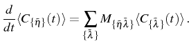
equations for
![]() can be equally found
applying the same QRF with
can be equally found
applying the same QRF with
![]() and a new set of
operators
and a new set of
operators
![]() where the previous operator
where the previous operator
![]() is included:
is included:
In the SE case, the initial state of these differential equations is the initial value of the correlators
In the general problem of two coupled modes, ![]() ,
, ![]() , we refer with
the label
, we refer with
the label
![]() to the two-time correlator
to the two-time correlator
![]() with
with
![]() , regardless
, regardless ![]() . This is the most general
form for the correlators, grouped in manifolds
. This is the most general
form for the correlators, grouped in manifolds
![]() . The
emission of particles
. The
emission of particles ![]() (
(![]() ) corresponds to
) corresponds to
![]() (
(![]() ). Each two-time correlator will have as initial condition
(
). Each two-time correlator will have as initial condition
(![]() ) the one-time correlator
) the one-time correlator
![]() (
(
![]() ) that belongs to the corresponding
manifold of the same order
) that belongs to the corresponding
manifold of the same order
![]() . The QRF for them,
with
. The QRF for them,
with
![]() , applies in a new set of operators
, applies in a new set of operators
![]() (
(
![]() ). The final result for the
correlator of interest,
). The final result for the
correlator of interest,
![]() , will be, as we
will see in the following Chapters, always of the form
, will be, as we
will see in the following Chapters, always of the form
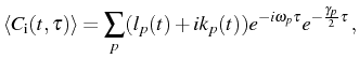
where all the new parameters, the weights
![$\displaystyle S_\mathrm{i}(\omega)=\frac1{\pi}\sum_{p}\left[L_p\frac{\frac{\gam...
...{\omega-\omega_p}{\big(\frac{\gamma_p}{2}\big)^2+(\omega-\omega_p)^2}\right]\,,$](img523.png)
which is in general a sum of many peaks labelled with
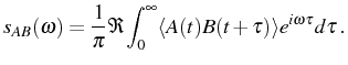
This way of computing the spectra, in which we take the Fourier
transform explicitly, gives us the structure of the lines in a
transparent way. ![]() and
and ![]() are the line positions and
broadenings. They originate from the energy levels structure and
uncertainties, whose skeleton is the Hamiltonian eigenstates, but that
can be greatly distorted by decoherence. As such, they are independent
of the channel of detection (cavity or direct exciton emission) and
independent of time. Coefficients
are the line positions and
broadenings. They originate from the energy levels structure and
uncertainties, whose skeleton is the Hamiltonian eigenstates, but that
can be greatly distorted by decoherence. As such, they are independent
of the channel of detection (cavity or direct exciton emission) and
independent of time. Coefficients ![]() and
and ![]() depend on the
one time correlators and, therefore, they are different in the SS or
the SE cases. They determine which lines actually appear in the
spectra, and with which intensity depending on the channel of emission
and the quantum state in the system.
depend on the
one time correlators and, therefore, they are different in the SS or
the SE cases. They determine which lines actually appear in the
spectra, and with which intensity depending on the channel of emission
and the quantum state in the system.
Most of the authors, like Savage (1989), Clemens et al. (2004), Porras & Tejedor (2003) or Perea et al. (2004), compute the spectrum with completely numerical methods from the density matrix and master equation. Their results are blind to the underlying individual lines and, therefore, miss all the information on the manifold structure that the spectra contains. This is a very dramatic loss if one is interested in quantum features or the crossover from quantum to classical regime, like in the case of this thesis. However, the lack of this information is not so important when the system is essentially classical or in the classical regime, where there is no quantized manifold structure. We should/will prefer this kind of ``blind'' methods then. In this direction and taking advantage of the SS properties, it is possible to go from the density matrix to the spectra without any need to compute the correlator. This method is described by Mølmer (1996) in his notes:
First, we choose a basis of states
![]() , ordered in a given
way and labelled with the index
, ordered in a given
way and labelled with the index
![]() . Then, we
obtain the density matrix, in its
. Then, we
obtain the density matrix, in its
![]() matrix form
matrix form
![]() , in the
SS. That is, we solve the master equation
, in the
SS. That is, we solve the master equation
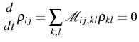
where
By means of the QRF, the spectrum can be put in terms of the matrix form of the operators
![$\displaystyle s_{AB}(\omega)=-\frac{1}{\pi}\Re\sum_{i,j,k,l,m}[(\mathcal{M}+i\omega I)^{-1}]_{ij,kl}\rho_{km}^{\mathrm{SS}} A_{ml}B_{ji}\,.$](img538.png)
Next: Second order correlation function Up: Theoretical Background Previous: The manifold approach Contents