The manifold approach

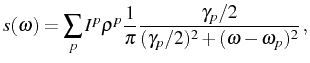
From the previous examples, we can generalize an approximate expression for the spectrum of emission that can give valuable and intuitive insights into the system under study. The spectra, in general, consist of a sum of peaks, at least one for each transition allowed in the system between energy levels. The peaks are specified by their lineshape, position, linewidth and intensity (or weight in the total spectrum). In Eq. (2.89) we can see that, for the case of Hamiltonian (2.66), the lineshape for each peak is a Delta function (with no broadening), positioned at $\omega_b+U(p-1)$ . Its weight in the total spectrum is given by the product of the population of state $\ket{p}$ , $\rho_{p}$ , times the probability of emission of such a state into the lower one $\ket{p-1}$ , $I^p=\vert\bra{p-1}a\ket{p}\vert^2=p$ , that is also the intensity of this transition [Eq. (2.5)]. If decay is considered, the lineshape becomes a Lorentzian, like in Eq. (2.93), or an other function depending on the interferences that can take place between the different transitions. In what follows of this Section, we will consider Lorentzian lineshapes for simplicity.

The extension of these ideas for a general system is what I have called the manifold method. It has been applied, for instance, by Laussy et al. (2006) and derived more rigorously by Vera et al. (2008) or Averkiev et al. (2009) from the exact expression for the spectra in Eq. (2.79). We assume that the total number of excitations is conserved by the Hamiltonian (the Hamiltonian dynamics take place inside each manifold independently), that the decay processes remove particles jumping between manifolds, and that the excitation mechanism does not change the energy structure. The method, based on the quantum jump approach, to obtain the elements of the approximate expression for the spectra

$\displaystyle s(\omega)=\sum_p I^p \rho^p \frac{1}{\pi}\frac{\gamma_p/2}{(\gamma_p/2)^2+(\omega-\omega_p)^2}\,,$

(2.95)

consists in the following steps:

Constructing a nonhermitian Hamiltonian that includes the decay of the modes in a complex frequency $\omega-i\gamma/2$ , by making the substitution (2.91). We know this Hamiltonian ultimately leads to unphysical results, but we also argued how it gives the correct ones for the average quantities of interest here.
Obtaining eigenenergies $\{E^k_i\}$ and eigenstates $\{\mathbf{e}^k_i\}$ of this Hamiltonian in a given manifold . We suppose that the system, in its coherent evolution, is in a superposition of these states.
The positions ( $\omega^k_{i,j}$ ) and broadenings ( $\gamma^k_{i,j}/2$ ) of the lines corresponding to each possible transition are given by, respectively, the imaginary and real parts of

$\displaystyle i[E^k_i-(E^{k-1}_j)^*]\,.$ (2.96)

This is simply because the positions are given by the difference in energy between the levels but the broadening of each line is given by the sum of the broadenings associated to them. The energy of the particle leaking out has an uncertainty given by the sum of the uncertainties in energy of the two levels.
Obtaining the amplitudes of probabilities of loosing an excitation from a given manifold to the neighboring one counting one excitation less. This is computed for each pair of states through the corresponding jump operator ( in the case of photon emission):

$\displaystyle I^{k\rightarrow k-1}_{i,j}=\vert\bra{k-1,j}a\ket{k,i}\vert^2\,.$ (2.97)
Obtaining $\rho^k_i$ , the average population of each state $\ket{k,i}$ , for example by solving the master equation.
Summing in Eq. (2.95) all the contributions $p\rightarrow \{k,i,j\}$ .

The resulting spectra is qualitatively similar to the exact results from Eq. (2.79) in the sense that it gives the good number of peaks and their positions in general. However, it is inaccurate in the broadenings and weights that are oversimplified. The whole picture breaks when the incoherent pump is comparable to the decay, as this is a strong source of decoherence, or when there are interferences between the different resonances and channels of emission of the system, as each transition is considered independently here. Therefore, although this method provides a good physical insight into the system and its spectra, we must also find a way to compute it exactly. The way forward to this is explained in the next Section.