Second order correlation function and the noise spectrum

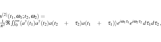
The power spectrum can only provide information on probabilities for single particles, being the Fourier transform of the first-order correlation function $G^{(1)}(t,\tau)$ . To investigate the statistics, we must go further in the order of the correlation functions. We already discussed the degree of second order coherence of a distribution, $g^{(2)}$ , in Eq. (2.7). Now we can generalize it to an arbitrary delay and define the two-time second-order correlation function:

$\displaystyle G^{(2)}(t,\tau)=\langle\ud{a}(t)\ud{a}(t+\tau)a(t+\tau)a(t)\rangle$

(2.109)

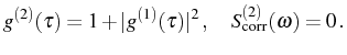
and its normalized version for stationary states, $g^{(2)}(t,\tau)=G^{(2)}(t,\tau)/\langle\ud{a}(t)a(t)\rangle ^2$ . $G^{(2)}(t,\tau)$ is related to the probability to emit two particles one after the other, at times

and $t+\tau$ , and it can also be identified with intensity correlations. Let us from now on consider that $t\rightarrow \infty$ and write expressions for the SS only, as this will be the most relevant case. As in the time domain, in order to fully describe the correlations between two particles emitted at different frequencies $\omega_1$ , $\omega_2$ , one would have to compute $S^{(2)}(\omega_1,\omega_2)=\langle\ud{a}(\omega_1)\ud{a}(\omega_2)a(\omega_2)a(\omega_1)\rangle /(n_a^\mathrm{SS})^2$ . Even more interesting is the two-photon counting resolved in frequency, which is related to a double Fourier transform

$\begin{multline} s^{(2)}(t_1,\omega_1;t_2,\omega_2)=\\ \frac{1}{\pi^2}\Re\iin... ...ngle e^{i\omega_1\tau_1}e^{i\omega_2\tau_2}\,d\tau_1d\tau_2 \,, \end{multline}$

in the SS (

). This is linked to the probability to detect the first photon at

with frequency $\omega_1$ and the second, at

with frequency $\omega_2$ . It is possible to obtain experimentally, integrating over some time and frequency windows, but quite technically involved in theory, as it requires at least three-time correlators (three implementations of the QRF). Therefore, we leave this for future investigations and, as a first approximation to the problem, we will simply analyze $S^{(2)}(\omega)\propto\int_{-\infty}^\infty s^{(2)}(\omega_1+\omega_a,\omega-\omega_1+\omega_a)d\omega_1$ . It corresponds to the Fourier transform

$\displaystyle S^{(2)}(\omega)=\frac{1}{\pi}\Re\int_0^\infty (g_\mathrm{SS}^{(2)}(\tau)-1)e^{i\omega\tau}\,d\tau \,,$

(2.110)

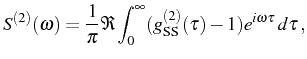
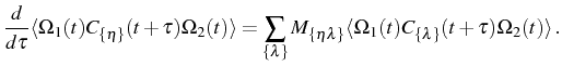
so it can be considered the intensity fluctuation spectrum or noise spectrum, in analogy with the power spectrum. $S^{(2)}(\omega)$ can also be interpreted as the joint density of probability that two particles in the system have frequencies whose fluctuations around the bare reference frequency ( $\omega_a$ ) sum up to $\omega$ . Still working with this simplified version of $S^{(2)}(\omega_1,\omega_2)$ , the two-particle frequency correlations are to be found in the difference between $S^{(2)}(\omega)$ and the convolution of individual densities of probability:

$\displaystyle S^{(2)}_\mathrm{corr}(\omega)=S^{(2)}(\omega)-\int_{-\infty}^\infty S(\omega_1+\omega_a)S(\omega-\omega_1+\omega_a)d\omega_1\,.$

(2.111)

The correlator $\langle\ud{a}(t)\ud{a}(t+\tau)a(t+\tau)a(t)\rangle$ needed here, can again be computed thanks to the QRF in the following way. Once Eq. (2.98) is satisfied for some set of operators $C_{\{\eta\}}$ , not only Eq. (2.99) holds, but also the relation

$\displaystyle \frac{d}{d\tau}\langle C_{\{\eta\}}(t+\tau)\Omega_2(t)\rangle =\s... ...{\lambda\}}M_{\{\eta\lambda\}}\langle C_{\{\lambda\}}(t+\tau)\Omega_2(t)\rangle$

(2.112)

is true for any general operator $\Omega_2$ , with the same regression matrix. From this, another useful equation involving two operators can be derived:

$\displaystyle \frac{d}{d\tau}\langle\Omega_1(t)C_{\{\eta\}}(t+\tau)\Omega_2(t)\... ...{\eta\lambda\}}\langle\Omega_1(t) C_{\{\lambda\}}(t+\tau)\Omega_2(t)\rangle \,.$

(2.113)

In the present case, we need to take $\Omega_1=\ud{a}$ and $\Omega_2=a$ , and find the set $C_{\{\eta\}}$ that includes the operator $\ud{a}a$ . It is interesting to note that the matrix of regression $M_{\{\eta\lambda\}}$ and the set of correlators $C_{\{\eta\}}$ involved in the computation of $G^{(2)}(t,\tau)$ are the same as those involved in the computation of the one-time average value

For the simple example of a thermal bosonic field, only the operators and $C_1=\ud{a}a$ are needed with $M_{1,1}=-\Gamma_a$ and $M_{1,0}=P_a$ . The result in the SS is $g^{(2)}(\tau)=1+e^{-\Gamma_a\tau}$ , that decays from (as it corresponds to the thermal SS) to the general infinite delay value of (two uncorrelated emissions). Thermal or chaotic sources correspond to the case where each emission event is independent and:

$\displaystyle g^{(2)}(\tau)=1+\vert g^{(1)}(\tau)\vert^2\,,\quad S^{(2)}_\mathrm{corr}(\omega)=0\,.$

(2.114)