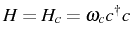
Basic examples

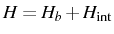
Before going further with the details on how to compute the two-time correlator and the power spectrum for a general system described by the master Eq. (2.71), we can try to learn on the basic structure and properties of these quantities through some basic examples. For the isolated modes, the two-time correlator can be obtained directly by solving the Heisenberg equations:

$\displaystyle \frac{d c}{dt}=i[H,c]$

(2.85)

for the creation/annihilation operators of the fields

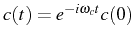
, $\sigma$ . A free mode ( $H=H_c=\omega_c \ud{c}c$ ), propagates like $c(t)=e^{-i\omega_c t}c(0)$ and therefore:

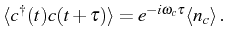$\displaystyle \langle\ud{c}(t)c(t+\tau)\rangle =e^{-i\omega_c\tau}\langle n_c\rangle \,.$

(2.86)

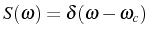
$\langle n_c\rangle$ is conserved and equal to the initial mean number of particles. The spectrum is therefore just a $\delta$ function, $S(\omega)=\delta(\omega-\omega_c)$ , with the pole at the energy of the mode $\omega_c$ . We can think of the spectrum of the Hamiltonian as the probability of emission when nothing is allowed to exit. The time uncertainty is very large, as we must wait an infinite time to detect a particle. The resonant energies are, therefore, exactly defined. They are given by the energy difference between eigenenergies of two consecutive manifolds. The emission spectrum is nothing else than the energy spectrum. We can see this with another example, adding interactions in the bosonic case, with the Hamiltonian of Eq. (2.66), $H=H_b+H_\mathrm{int}$ . Note that

and therefore $n_b=\ud{b}b$ is a constant of motion. Then, the operator

depends on the manifold as

$\displaystyle b(t)=e^{-i(\omega_b +U n_b)t}b(0)\,,$

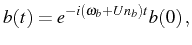(2.87)

and so does the correlator:

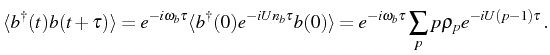$\displaystyle \langle\ud{b}(t)b(t+\tau)\rangle =e^{-i\omega_b\tau}\langle\ud{b}... ...-iU n_b\tau}b(0)\rangle =e^{-i\omega_b\tau}\sum_p p\rho_{p} e^{-iU(p-1)\tau}\,.$

(2.88)

This yields a spectrum for the

operator,

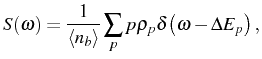$\displaystyle S(\omega)=\frac{1}{\langle n_b\rangle }\sum_p p \rho_{p}\delta\big(\omega-\Delta E_p\big)\,,$

(2.89)

which simply weights with the occupation ( $\rho_{p}$ ) and the intensity

, the resonances that corresponds to transitions between each consecutive pair of manifolds:

$\displaystyle \Delta E_p=\bra{p}H\ket{p}-\bra{p-1}H\ket{p-1}=\omega_b+U(p-1)\,.$

(2.90)

When the lifetime of the particles in the system is not infinite, the uncertainty in the energy of the emitted particle increases. This corresponds to changing the $\delta$ functions by a broadened function with a linewidth. One can think naively and simply break the conservation of particles by adding some exponential decay to the operators $c(t)=e^{-i\omega_c t}e^{-\frac{\gamma_c}{2}t}c(0)$ which results in the expected decay of particles $\langle n_c\rangle (t)=e^{-\gamma_c t}\langle n_c\rangle (0)$ . This corresponds--and it is often found in the literature--to adding an imaginary part to the energy

$\displaystyle \omega_c\rightarrow\omega_c-i\frac{\gamma_c}{2}$

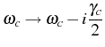(2.91)

in the free Hamiltonian

and solving the equation $d c/dt=-i\omega_c c-\gamma_c/2 c$ . This procedure is in general incorrect. This was made clear, for instance, by Yamamoto & Imamoglu (1999). It leads to unphysical results like the decay of the bosonic commutation relation: $[a(t),\ud{a}(t)]=e^{-\gamma t}$ . Dissipation not only empties the system but also induces quantum noise due to fluctuations in the reservoir. 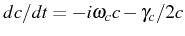A more elaborated method is needed, such as a master equation with Lindblad terms, that we presented in Section 2.4. 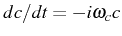Equivalently, the Heisenberg equations for the operators $d c/dt=-i\omega_c c$ can be upgraded to the quantum Langevin equations,

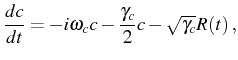$\displaystyle \frac{d c}{dt}=-i\omega_c c-\frac{\gamma_c}{2} c-\sqrt{\gamma_c}R(t)\,,$

(2.92)

where the quantum white noise operator

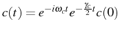
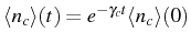
is introduced. This operator is determined by the state of the bath. The average value of its commutation relations carries the statistic information which leads to the expected physical results. However, depending on the system, solving the Heisenberg equations with decay introduced as an imaginary frequency, can give rise to the same results as solving the Langevin equations. 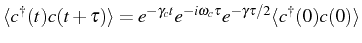For example, in the case of averaged quantities like $\langle n_c\rangle$ or the two-time correlator, $\langle\ud{c}(t)c(t+\tau)\rangle =e^{-\gamma_c t}e^{-i\omega_c \tau}e^{-\gamma \tau /2}\langle\ud{c}(0)c(0)\rangle$ , the correct expression is obtained. Before we derive them using the proper methods, let us just write the spectrum this yields:

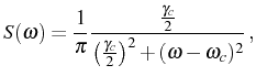$\displaystyle S(\omega)=\frac{1}{\pi}\frac{\frac{\gamma_c}2}{\big(\frac{\gamma_c}2\big)^2+(\omega-\omega_c)^2}\,,$

(2.93)

where we used

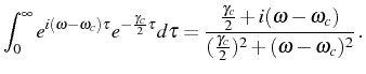$\displaystyle \int_0^\infty e^{i(\omega-\omega_c)\tau}e^{-\frac{\gamma_c}2\tau}... ...rac{\gamma_c}2+i(\omega-\omega_c)}{(\frac{\gamma_c}2)^2+(\omega-\omega_c)^2}\,.$

(2.94)

This is the Cauchy-Lorentz distribution with a full width at half its maximum (FWHM) given by $\gamma_c$ , which is also the inverse lifetime of the particles in the system. This shape is the most commonly found in spectroscopy as it appears when the mechanisms causing the broadening of the line affects homogeneously all the emitters.