

Next: Population and Statistics Up: The Jaynes-Cummings model Previous: First order correlation function Contents
Vanishing pump case in the manifold picture
In this Section, we discuss the series of parameters ![]() and
and ![]() that in the luminescence spectrum,
Eq. (5.25), determine the position and the
broadening (FWHM) of the lines, respectively, in both the cavity and
the direct exciton emission. The case of vanishing pumping is
fundamental, as it corresponds to the textbook Jaynes-Cummings results
with the SE of an initial state. It serves as the skeleton for the
general case with arbitrary pumping and supports the general physical
picture. Finally, it admits analytical results. We therefore begin
with the case where
that in the luminescence spectrum,
Eq. (5.25), determine the position and the
broadening (FWHM) of the lines, respectively, in both the cavity and
the direct exciton emission. The case of vanishing pumping is
fundamental, as it corresponds to the textbook Jaynes-Cummings results
with the SE of an initial state. It serves as the skeleton for the
general case with arbitrary pumping and supports the general physical
picture. Finally, it admits analytical results. We therefore begin
with the case where
![]() . The
eigenvalues of the matrix of regression
. The
eigenvalues of the matrix of regression
![]() , are grouped into
manifolds. There are two for the first manifold, given by:
, are grouped into
manifolds. There are two for the first manifold, given by:
and four for each manifold of higher order
in terms of the
and of the
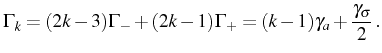
For each manifold, we have defined the
![\includegraphics[width=.95\linewidth]{chap5/JC/fig2-ladder.eps}](img1525.png) |
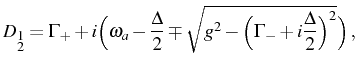
According to Eq. (5.24), these provide the
position ![]() of the line and its half-broadening
of the line and its half-broadening
![]() through their imaginary and real parts.
through their imaginary and real parts. ![]() is always real, so
it contributes in all cases to
is always real, so
it contributes in all cases to ![]() only.
only. ![]() is (at
resonance) either pure real, or pure imaginary, and similarly to the
LM or the two coupled 2LSs, this is what defines SC. This corresponds
to an oscillatory or damped field dynamics of the two-time correlators
within manifold
is (at
resonance) either pure real, or pure imaginary, and similarly to the
LM or the two coupled 2LSs, this is what defines SC. This corresponds
to an oscillatory or damped field dynamics of the two-time correlators
within manifold ![]() , which lead us to the formal definition: WC and SC
of order
, which lead us to the formal definition: WC and SC
of order ![]() are defined as the regime where the complex Rabi
frequency at resonance, Eq. (5.28), is pure
imaginary (WC) or real (SC). The criterion for
are defined as the regime where the complex Rabi
frequency at resonance, Eq. (5.28), is pure
imaginary (WC) or real (SC). The criterion for ![]() th order SC is
therefore:
th order SC is
therefore:
SC is achieved more easily, given the system parameters (![]() and
and
![]() ), with an increasing photon-field intensity
that enhances the effective coupling strength. The lower the SC order,
the stronger the coupling. This corresponds to the
), with an increasing photon-field intensity
that enhances the effective coupling strength. The lower the SC order,
the stronger the coupling. This corresponds to the ![]() th manifold
(and all above) being in SC (aided by the cavity photons), while the
th manifold
(and all above) being in SC (aided by the cavity photons), while the
![]() manifolds below are in WC. First order is therefore the one
where all manifolds are in SC. Eq. (5.30)
includes the standard SC of the LM and 2LSs,
manifolds below are in WC. First order is therefore the one
where all manifolds are in SC. Eq. (5.30)
includes the standard SC of the LM and 2LSs,
![]() , as the
first order SC of the fermion case, that is shown in green (thick) in
Fig. 5.12 (see also and compare with
Fig. 3.1 for bosons). The same position of
the peaks
, as the
first order SC of the fermion case, that is shown in green (thick) in
Fig. 5.12 (see also and compare with
Fig. 3.1 for bosons). The same position of
the peaks
![]() and the same (half)
broadenings
and the same (half)
broadenings
![]() is also recovered (in the absence of
pumping). Note that similarly to the boson case, the SC is defined by
a comparison between the coupling strenght
is also recovered (in the absence of
pumping). Note that similarly to the boson case, the SC is defined by
a comparison between the coupling strenght ![]() with the
difference of the effective broadening
with the
difference of the effective broadening ![]() and
and ![]() . The sum of these play no role in this regard.
. The sum of these play no role in this regard.
The ![]() and
and
![]() are plotted in
Fig. 5.12(a) and
5.12(b), respectively, as function
of
are plotted in
Fig. 5.12(a) and
5.12(b), respectively, as function
of ![]() . Note that
. Note that ![]() only depends on
only depends on ![]() and
and
![]() , whereas
, whereas ![]() also depends on
also depends on ![]() (that is why
we plot it for
(that is why
we plot it for
![]() ).
).
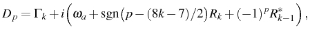
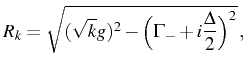
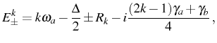
The ![]() , Eq. (5.27), have a natural
interpretation in terms of transitions between the manifolds of the
so-called Jaynes-Cummings ladder. The eigenenergies of the
Jaynes-Cummings Hamiltonian with decay granted as the imaginary part
of the bare energies (
, Eq. (5.27), have a natural
interpretation in terms of transitions between the manifolds of the
so-called Jaynes-Cummings ladder. The eigenenergies of the
Jaynes-Cummings Hamiltonian with decay granted as the imaginary part
of the bare energies (
![]() ), are
given by
), are
given by ![]() with
with
 |
(5.31) |
for the
![\begin{subequations}\begin{align}&D_{4k-5}=i[E^k_--(E^{k-1}_+)^*]\, ,\quad &D_{4...
...+)^*]\, ,\quad &D_{4k-2}=i[E^k_+-(E^{k-1}_-)^*]\,. \end{align}\end{subequations}](img1535.png)
In the case
The ladder is shown (at resonance) in
Fig. 5.12(c) in the same way as we
reconstructed it for bosons in
Fig. 3.1. Let us discuss it in connection
with our definition of SC in this system, to arbitrary ![]() . When
. When
![]() , each step of the ladder is constituted by the two
eigenstates of the fermion, dressed by the
, each step of the ladder is constituted by the two
eigenstates of the fermion, dressed by the ![]() cavity photons,
resulting in a splitting of
cavity photons,
resulting in a splitting of
![]() . This kind of renormalization
already appeared in Chapter 4 when we discussed the
coupled two 2LSs, that can be considered as a particular case of the
JCM, where there can be no more than a photon in the system. An
. This kind of renormalization
already appeared in Chapter 4 when we discussed the
coupled two 2LSs, that can be considered as a particular case of the
JCM, where there can be no more than a photon in the system. An
![]() -dependent splitting produces quadruplets of delta peaks with
splitting of
-dependent splitting produces quadruplets of delta peaks with
splitting of
![]() around
around ![]() , as
opposed to the LM where independently of the manifold, the peaks are
all placed at
, as
opposed to the LM where independently of the manifold, the peaks are
all placed at ![]() around
around ![]() . In a more general situation
with
. In a more general situation
with
![]() , there are three possibilities for a
manifold
, there are three possibilities for a
manifold ![]() :
:
- Both manifold
 and
and  are in SC. The two Rabi
coefficients
are in SC. The two Rabi
coefficients  and
and  are real. This is the case when
The luminescence spectra corresponds to four splitted lines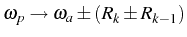 , coming from
the four possible transitions
[Eqs. (5.32), shown as
, coming from
the four possible transitions
[Eqs. (5.32), shown as  and
and  in
Fig. 5.12(c)] between manifolds
and . The emission from all the higher manifolds also produces
four lines. They are grouped pairwise around
in
Fig. 5.12(c)] between manifolds
and . The emission from all the higher manifolds also produces
four lines. They are grouped pairwise around  [Fig. 5.12(a)] and all have the same
broadening, contributed by
[Fig. 5.12(a)] and all have the same
broadening, contributed by  only [the single straight line
in Fig. 5.12(b)].
only [the single straight line
in Fig. 5.12(b)].
- Manifold is in SC while manifold is in WC. In
this case, is pure imaginary (contributing to line positions)
and is real (contributing to broadenings). This is the
case when
This corresponds to two lines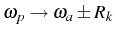 in the luminescence spectrum, coming from the two possible
transitions [shown as
in the luminescence spectrum, coming from the two possible
transitions [shown as  in
Fig. 5.12(c)] between the SC
manifold and the WC manifold . Each of them is doubly
degenerated. The two contributions at a given
in
Fig. 5.12(c)] between the SC
manifold and the WC manifold . Each of them is doubly
degenerated. The two contributions at a given  have two
distinct broadenings
have two
distinct broadenings
 around . [cf. Fig. 5.12(b)]. The
final lineshapes of the two lines
around . [cf. Fig. 5.12(b)]. The
final lineshapes of the two lines  is the same. In this region,
all the emission from the higher manifolds produce four lines and
all from the lower produce only one (at ), being in WC.
is the same. In this region,
all the emission from the higher manifolds produce four lines and
all from the lower produce only one (at ), being in WC.
- Both manifold and are in WC. The two Rabi
coefficients and are pure imaginary. This is the
case when
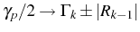
This corresponds to only one line at in the luminescence spectrum, coming from the transition from one
manifold in WC to the other [shown as
in the luminescence spectrum, coming from the transition from one
manifold in WC to the other [shown as  in
Fig. 5.12(c)]. The line is four-time
degenerated, with four contributions with different
broadenings
in
Fig. 5.12(c)]. The line is four-time
degenerated, with four contributions with different
broadenings
 , as seen in Fig. 5.12(b).
Figure 5.12 is the skeleton for the luminescence spectra--whether that of the cavity or of the direct exciton emission. It specifies at what energies can be the possible lines that constitutes the final lineshape, and what are their broadening. To compose the final result, we only require to know the weight of each of these lines.
In the SE case, the weights ![]() and
and ![]() include the integral of
the single-time mean values
include the integral of
the single-time mean values
![]() over
over
![]() . Therefore, only those manifolds with a smaller number of
excitations than the initial state can appear in the spectrum. Each of
them, will be weighted by the specific dynamics of the system. The
``spectral structure''--i.e., the
. Therefore, only those manifolds with a smaller number of
excitations than the initial state can appear in the spectrum. Each of
them, will be weighted by the specific dynamics of the system. The
``spectral structure''--i.e., the ![]() and
and ![]() --depends
only the system parameters (
--depends
only the system parameters (![]() and
and
![]() ). Therefore,
in the SE case, the resulting emission spectrum is an exact mapping of
the spectral structure of the Hamiltonian,
Fig. 5.12.
). Therefore,
in the SE case, the resulting emission spectrum is an exact mapping of
the spectral structure of the Hamiltonian,
Fig. 5.12.
In the SS case, the weighting of the lines also depends on which
quantum state is realized, this time under the balance of pumping and
decay. But the excitation scheme also changes the spectral structure
of Fig. 5.12. When the pumping parameters
are small, the changes will mainly be perturbations of the present
picture and most concepts will still hold, such as the definition of
SC, Eq. (5.30) for nonzero
![]() in (5.17). However, when the pump
parameters are comparable to the decay parameters, the manifold
picture in terms of Hamiltonian eigenenergies breaks, as it happen for
the two coupled 2LS in Chapter 4. The underlying
spectral structure must be computed numerically for each specific
probing of the system with
in (5.17). However, when the pump
parameters are comparable to the decay parameters, the manifold
picture in terms of Hamiltonian eigenenergies breaks, as it happen for
the two coupled 2LS in Chapter 4. The underlying
spectral structure must be computed numerically for each specific
probing of the system with ![]() and
and ![]() . It can still be
possible to identify the origin of the lines with the manifold
transitions by plotting their position
. It can still be
possible to identify the origin of the lines with the manifold
transitions by plotting their position ![]() as a function of the
pumps, starting from the analytic limit. SC of each manifold can be
associated to the existence of peaks positioned at
as a function of the
pumps, starting from the analytic limit. SC of each manifold can be
associated to the existence of peaks positioned at
![]() . We address this problem in next Sections.
. We address this problem in next Sections.
Next: Population and Statistics Up: The Jaynes-Cummings model Previous: First order correlation function Contents