Mean values
Let us start by introducing the notations that will be useful in the general description of SE and SS emission. The effective broadenings reduce to the decay rates in the SE case but get renormalized by the pumping rate in the SS case:
We shall also use thoroughly the combinations:
Thanks to the general relations
![]() and
and
![]() , we can
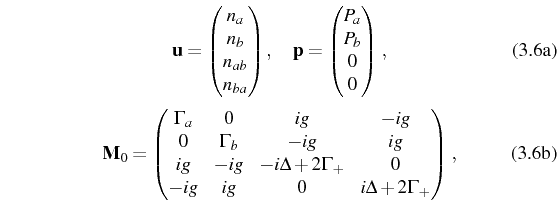
obtain from Eq. (3.3) the single-time mean values of interest
for this problem, by solving the equation of motion of the coupled
system:
, we can
obtain from Eq. (3.3) the single-time mean values of interest
for this problem, by solving the equation of motion of the coupled
system:
with
where
The solution,
gives the cavity population:
The expression for ![]() follows from
follows from
![]() . The
crossed mean value that reflects the coherent coupling reads:
. The
crossed mean value that reflects the coherent coupling reads:
where we have defined the complex (half) Rabi frequency:
that arises as a direct extension of the dissipationless case, Eq. (2.56c).
![\includegraphics[width=0.3\linewidth]{chap3/newFigs/boson.ps}](img615.png) |
It is of interest to note that Eqs. (3.10)-(3.11)
are reproduced by introducing decay as an imaginary part to the
energies in the Heisenberg picture, i.e., substituting
![]() by
by
![]() and solving directly in a full
Hamiltonian picture the operator equations of
motion:
and solving directly in a full
Hamiltonian picture the operator equations of
motion:
![]() with
with ![]() . This method goes along the
lines of the manifold picture (closely related to the Langevin
equations), represented in
Fig. 3.1. Although essentially incorrect
(as we explained in the previous Chapter), following this method
provides the right average quantities, such as the correlator
. This method goes along the
lines of the manifold picture (closely related to the Langevin
equations), represented in
Fig. 3.1. Although essentially incorrect
(as we explained in the previous Chapter), following this method
provides the right average quantities, such as the correlator
![]() and therefore leads also to the correct
expression for the SE spectra. The expressions that we obtain for the
four time-dependent operators (
and therefore leads also to the correct
expression for the SE spectra. The expressions that we obtain for the
four time-dependent operators (![]() ,
, ![]() ,
, ![]() ,
,
![]() ) solving the Heisenberg (not the Langevin!) equations are all
contained in:
) solving the Heisenberg (not the Langevin!) equations are all
contained in:
The operators at zero time,
On the other hand, the SS case corresponds to setting the time derivative on the left hand side of Eq. (3.6) to zero, and solving the resulting set of linear equations. The solution
explicitly yields:
Both photonic and excitonic reduced density matrices are diagonal. They correspond to thermal distributions of particles with the above mean numbers:
Behind their forbidding appearance,
Eqs. (3.15) enjoy a transparent physical
meaning, that they inherit from the semi-classical--and therefore
intuitive--picture of rate equations. When the coupling strength
between the two modes, ![]() , vanishes, the solutions are those of
thermal equilibrium for
, vanishes, the solutions are those of
thermal equilibrium for ![]() and
and ![]() [Eqs. (2.34)
and (2.52)]. In the general case
where
[Eqs. (2.34)
and (2.52)]. In the general case
where ![]() , the mean numbers can also be written in the same form:
, the mean numbers can also be written in the same form:
(Id. for mode
with
in terms of the effective coupling strength at nonzero detuning:
From the point of view of mode ![]() , the coupling with mode
, the coupling with mode ![]() is both
adding particles, contributing to
is both
adding particles, contributing to
![]() , and removing
them, contributing to
, and removing
them, contributing to
![]() . The total effective
decay is:
. The total effective
decay is:
Note that the generalized Purcell rate
The mean value of the coherence can also be expressed in terms of these quantities:
where
The quantities defined in Eqs. (3.18) and
Eq. (3.21) are all positive when
![]() (
(![]() ) and all negative when
) and all negative when
![]() (if there
exists a solution for the steady state). The conditions for the
pumping terms
(if there
exists a solution for the steady state). The conditions for the
pumping terms ![]() ,
, ![]() to yield a physical state (a steady state),
are therefore those for which the mean values
to yield a physical state (a steady state),
are therefore those for which the mean values
![]() are positive and finite, implying:
are positive and finite, implying:
The first condition requires that pumps
From now on, we shall refer with ``SE'' and ``SS'' to the expressions
that apply specifically to the spontaneous emission and to the steady
state, respectively, leaving free of index those that are of general
validity. In some cases, as for instance in
Eq. (3.4), no index is required if it is
understood that ![]() are defined and equal to zero in the SE
case. For that reason, we shall leave
are defined and equal to zero in the SE
case. For that reason, we shall leave ![]() free of the SE/SS
redundant index.
free of the SE/SS
redundant index.
Elena del Valle ©2009-2010-2011-2012.


 and
and


![$\displaystyle \Big[\cos{(R_\mathrm{r} t)}+\cosh{(R_\mathrm{i} t})\Big]\frac{n_a^0}{2}$](img593.png)
![$\displaystyle \Big[\cos{(R_\mathrm{r}t)}-\cosh{(R_\mathrm{i} t)}\Big]\frac{(\fr...
...+ g^2 n_b^0+ g \Delta \Re{n_{ab}^0}-2g \gamma_- \Im{n_{ab}^0}}{2\vert R\vert^2}$](img595.png)
![$\displaystyle \left[\frac{\sin{(R_\mathrm{r} t)}}{R_\mathrm{r}}+\frac{\sinh{(R_\mathrm{i}t})}{R_\mathrm{i}} \right]\left( g \Im{n_{ab}^0}-\gamma_- n_a^0 \right)$](img597.png)

![$\displaystyle n_{ab}(t)=e^{-2 \gamma_+ t}\Bigg\{\Big[\cos{(R_\mathrm{r} t)}+\cosh{(R_\mathrm{i} t})\Big]\frac{n_{ab}^0}{2}$](img601.png)
![$\displaystyle \Big[\cos{(R_\mathrm{r} t)}-\cosh{(R_\mathrm{i} t)}\Big]\frac{g(\...
..._b^0-(\frac{\Delta^2}{4}+\gamma_-^2) n_{ab}^0+g^2(n_{ab}^0)^*}{2\vert R\vert^2}$](img602.png)
![$\displaystyle \left[\frac{\sin{(R_\mathrm{r} t)}}{R_\mathrm{r}}+\frac{\sinh{(R_\mathrm{i} t})}{R_\mathrm{i}} \right]\frac{i(\Delta n_{ab}^0-g(n_a^0-n_b^0))}{2}$](img603.png)
![$\displaystyle \left[\frac{\sin{(R_\mathrm{r} t)}}{R_\mathrm{r}}-\frac{\sinh{(R_\mathrm{i} t})}{R_\mathrm{i}} \right]\times$](img604.png)


![\begin{multline}
a(t)=e^{-(\gamma_+-i\frac{\Delta}{2})t}\Big[ e^{iRt}
\frac{...
...Rt}
\frac{(R-i\gamma_++\frac{\Delta}{2})a(0)+g b(0)}{2R}\Big]\,.
\end{multline}](img622.png)


