

Next: Vanishing pump case in Up: The Jaynes-Cummings model Previous: The Jaynes-Cummings model Contents
First order correlation function and power spectrum
In the LM, the symmetry
![]() allowed to focus
exclusively on the cavity-emission without loss of generality, as the
direct exciton emission could be obtained from the cavity emission by
interchanging parameters. Here, the exciton (fermion) and photon
(boson) are intrinsically different, and no simple relationship links
them. They must therefore be computed independently. In order to apply
the QRF (2.99), four indices are required to
label the closing operators, namely
allowed to focus
exclusively on the cavity-emission without loss of generality, as the
direct exciton emission could be obtained from the cavity emission by
interchanging parameters. Here, the exciton (fermion) and photon
(boson) are intrinsically different, and no simple relationship links
them. They must therefore be computed independently. In order to apply
the QRF (2.99), four indices are required to
label the closing operators, namely
![]() in
in
![]() with
with ![]() ,
,
![]() and
and ![]() ,
,
![]() . The links established
between them by the Liouvillian dynamics are given the rules:
. The links established
between them by the Liouvillian dynamics are given the rules:
and zero everywhere else. We are interested in
The links between the various correlators tracked through the
indices ![]() , are shown in
Fig. 5.11. It is very interesting to
compare this schema with those of the LM
(Fig. 3.2), the two coupled 2LSs
(Fig. 4.2) and the AO
(Fig. 5.1). We can easily distinguish the
models that can be solved analytically from the fact that a manifold
, are shown in
Fig. 5.11. It is very interesting to
compare this schema with those of the LM
(Fig. 3.2), the two coupled 2LSs
(Fig. 4.2) and the AO
(Fig. 5.1). We can easily distinguish the
models that can be solved analytically from the fact that a manifold
![]() of the schema does not ``call'' higher ones
of the schema does not ``call'' higher ones ![]() . In the LM, this
is due to a natural truncation. The first manifolds
. In the LM, this
is due to a natural truncation. The first manifolds
![]() and
and
![]() , in green, are enough to compute the
spectra and populations. In the two 2LSs, the reason of truncation is
the saturation of both dots, that reduces the number of nonzero
correlators to a few (all nonzero one-time correlators are in the
graph). In this case, the first but also the second manifold are
involved in the spectra.
, in green, are enough to compute the
spectra and populations. In the two 2LSs, the reason of truncation is
the saturation of both dots, that reduces the number of nonzero
correlators to a few (all nonzero one-time correlators are in the
graph). In this case, the first but also the second manifold are
involved in the spectra.
![]() and
and
![]() are smaller than for the JC, again reduced by saturation of the second
mode. The second manifold in general differs for each model. As we
know, the models only converge in the first manifold that corresponds
to the linear regime. The AO and the JCM both require an external
truncation to close their equations. In the AO, it is the interaction
who links the manifolds to higher ones while in the JCM, it is the
coupling. SE imposes a truncation at the highest manifold that the
initial state involves.
are smaller than for the JC, again reduced by saturation of the second
mode. The second manifold in general differs for each model. As we
know, the models only converge in the first manifold that corresponds
to the linear regime. The AO and the JCM both require an external
truncation to close their equations. In the AO, it is the interaction
who links the manifolds to higher ones while in the JCM, it is the
coupling. SE imposes a truncation at the highest manifold that the
initial state involves.
To solve the differential equations of motion in
Eq. (2.99), the initial value of each
correlator is also required, e.g.,
![]() demands
demands
![]() , etc. The initial values of
, etc. The initial values of
![]() (resp.,
(resp.,
![]() ) can be conveniently computed
within the same formalism, recurring to
) can be conveniently computed
within the same formalism, recurring to
![]() and
and
![]() with
with
![]() (resp.,
(resp.,
![]() ). This allows to compute also the single-time
dynamics
). This allows to compute also the single-time
dynamics
![]() , and their steady
state, from the same tools used as for the two-time dynamics through
the QRF. The indices
, and their steady
state, from the same tools used as for the two-time dynamics through
the QRF. The indices
![]() required for the single-time
correlators form a set--that we call
required for the single-time
correlators form a set--that we call
![]() --that is
disjoint from
--that is
disjoint from
![]() , required for the
two-times dynamics. The set
, required for the
two-times dynamics. The set
![]() has--beside the
constant term
has--beside the
constant term
![]() --two more elements for the lower
manifold (of the LM). This is because
--two more elements for the lower
manifold (of the LM). This is because
![]() and
and
![]() invoke
invoke ![]() and
and ![]() for
the cavity spectrum on the one hand, and
for
the cavity spectrum on the one hand, and ![]() and
and ![]() for the exciton emission on the other. At higher orders
for the exciton emission on the other. At higher orders ![]() , all
two-times correlators
, all
two-times correlators
![]() otherwise depend on the same
four single-time correlators
otherwise depend on the same
four single-time correlators
![]() . Independently of
which spectrum one wishes to compute, these four elements
. Independently of
which spectrum one wishes to compute, these four elements ![]() ,
,
![]() ,
, ![]() and
and ![]() of
of
![]() are needed in all cases as they are linked to each other, as shown in
Fig. 5.11.
are needed in all cases as they are linked to each other, as shown in
Fig. 5.11.
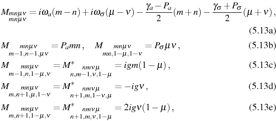
In the figure, only the type of coupling--coherent, through ![]() , or
incoherent, through the pumpings
, or
incoherent, through the pumpings
![]() --has been
represented. Weighting coefficients are given by
Eqs. (5.14). Of particular relevance is the
self-coupling of each correlator to itself, not shown on the figure
for clarity. Its coefficient, Eq. (5.14a),
lets enter
--has been
represented. Weighting coefficients are given by
Eqs. (5.14). Of particular relevance is the
self-coupling of each correlator to itself, not shown on the figure
for clarity. Its coefficient, Eq. (5.14a),
lets enter
![]() that do not otherwise couple any one
correlator to any of the others. This makes it possible to describe
decay, at vanishing pump, with the manifold method by simply providing
an imaginary part to the Energy in
Eq. (5.11). The incoherent pumping, on the
other hand, establishes a new set of connections between
correlators. Note, however, that at the exception of
that do not otherwise couple any one
correlator to any of the others. This makes it possible to describe
decay, at vanishing pump, with the manifold method by simply providing
an imaginary part to the Energy in
Eq. (5.11). The incoherent pumping, on the
other hand, establishes a new set of connections between
correlators. Note, however, that at the exception of
![]() , the
pumping does not enlarge the sets
, the
pumping does not enlarge the sets
![]() ,
,
![]() : the structure remains the same (also,
technically, the computational complexity is identical), only with the
correlators affecting each other differently. The addition
of
: the structure remains the same (also,
technically, the computational complexity is identical), only with the
correlators affecting each other differently. The addition
of
![]() by the pumping terms bring the same additional physics
in the boson and fermion cases: it imposes a self-consistent steady
state over a freely chosen initial condition. In the LM, the pumping
had otherwise only a direct influence in renormalizing the
self-coupling of each correlator. In the JCM, it brings direct
modifications to the Hamiltonian coherent dynamics. But its
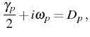
contribution to the self-coupling is also important, and gives rise to
an interesting fermionic opposition to the bosonic effects as seen in
Eq. (5.14a) in the effective linewidth:
by the pumping terms bring the same additional physics
in the boson and fermion cases: it imposes a self-consistent steady
state over a freely chosen initial condition. In the LM, the pumping
had otherwise only a direct influence in renormalizing the
self-coupling of each correlator. In the JCM, it brings direct
modifications to the Hamiltonian coherent dynamics. But its
contribution to the self-coupling is also important, and gives rise to
an interesting fermionic opposition to the bosonic effects as seen in
Eq. (5.14a) in the effective linewidth:
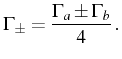
For later convenience, we also define:
Eq. (5.16), reminds us that, whereas the incoherent cavity pumping narrows the linewidth, as a manifestation of its boson character, the incoherent exciton pumping broadens it. This opposite tendencies, participating together in the dynamics, bear a capital importance for the lineshapes, as narrow lines favor the observation of a structure, whereas broadening hinders it. On the other hand, the cavity incoherent pumping always results in a thermal distribution of photons with large fluctuations of the particle numbers, that brings inhomogeneous broadening, whereas the exciton pumping can grow a Poisson-like distribution with little fluctuations. Both types of pumping, however, ultimately bring decoherence to the dynamics and induce the transition into WC, with the lines composing the spectrum collapsing into one. Putting all these effects together, there is an optimum configuration of pumpings where particle fluctuations compensate for the broadening of the interesting lines, enhancing their resolution in the spectrum, as we shall see when we discuss the results below.
As there is no finite closure relation, some truncation is in
order. We will adopt the same scheme as for the AO, where a maximum
of
![]() excitation(s) (photon plus excitons) is considered
at the
excitation(s) (photon plus excitons) is considered
at the
![]() th order, thereby truncating by manifolds of
correlators, which is the most relevant picture. This means that the
last manifold considered in Fig. 5.11
is
th order, thereby truncating by manifolds of
correlators, which is the most relevant picture. This means that the
last manifold considered in Fig. 5.11
is
![]() , the one with mean values indexes that
fit
, the one with mean values indexes that
fit
![]() . The exact result is recovered in
the limit
. The exact result is recovered in
the limit
![]() . As seen in
Fig. 5.11, the number
. As seen in
Fig. 5.11, the number
![]() of
two-time correlators from
of
two-time correlators from
![]() up to order
up to order
![]() is
is
![]() and the number of mean values
from
and the number of mean values
from
![]() is
is
![]() . The problem is
therefore computationally linear in the number of excitations, and as
such is as simple as it could be for a quantum system. The general
case consists in a linear system of
. The problem is
therefore computationally linear in the number of excitations, and as
such is as simple as it could be for a quantum system. The general
case consists in a linear system of
![]() coupled
differential equations, whose matrix of coefficients [specified by
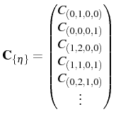
Eqs. (5.14)] is, in the basis
of
coupled
differential equations, whose matrix of coefficients [specified by
Eqs. (5.14)] is, in the basis
of
![]() , a
, a
![]() square matrix
that we denote
square matrix
that we denote
![]() . With these definitions, the quantum
regression theorem becomes:
. With these definitions, the quantum
regression theorem becomes:
where
 and
and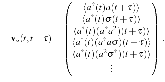
The ordering of the correlators is arbitrary. We fix it to that of Fig. 5.11, as seen in Eq. (5.19). With this convention, the indices of the two correlators of interests are:
![\includegraphics[width=.9\linewidth]{chap5/JC/fig1-correlator.ps}](img1491.png) |
To solve Eq. (5.18), we introduce the
matrix
![]() of normalized eigenvectors of
of normalized eigenvectors of
![]() ,
and
,
and
![]() the diagonal matrix of eigenvalues:
the diagonal matrix of eigenvalues:
The formal solution is given by
![]() .
Integration of
.
Integration of
![]() and
application of the Wiener-Khintchine formula yield for the
and
application of the Wiener-Khintchine formula yield for the ![]() th and
th and
![]() th rows of
th rows of
![]() the emission spectra of the
cavity, namely,
the emission spectra of the
cavity, namely,
![]() on the one hand,
and of the direct exciton emission,
on the one hand,
and of the direct exciton emission,
![]() , on the other hand. We find, to
order
, on the other hand. We find, to
order
![]() :
:
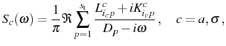
where
![$\displaystyle L^c_{i_cp}+iK^c_{i_cp}=\frac1{n_c}[\mathbf{E}]_{i_cp}\sum_{q=1}^{...
...}}[\mathbf{E}^{-1}]_{pq}[\mathbf{v}_c(t,t)]_q\,,\quad 1\le p\le s_\mathrm{t}\,,$](img1506.png)
and
we can write Eq. (5.22) in a less concise but more transparent way. To all orders, it reads:
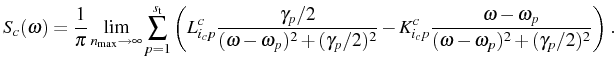
The lineshape, as in all the models we have studied in this thesis, is composed of a series of Lorentzian and Dispersive parts, whose positions and broadenings (FWHM) are specified by
Next: Vanishing pump case in Up: The Jaynes-Cummings model Previous: The Jaynes-Cummings model Contents