Population and Statistics

To know which features of the spectral structure dominate and which are negligible, one needs to know what is the quantum state of the system. In the LM, it was enough to know the average photon () and exciton () numbers, and the off-diagonal element $n_{ab}=\langle\ud{a}b\rangle$ . In the two 2LS, only one more averaged quantity, , was necessary. In the most general case of the fermion system, a countably infinite number of parameters are required for the exact lineshape, as in the LM with interactions or the AO. The new order of complexity brought by the fermion system is illustrated for even the simplest observable. Instead of a closed relationship that provides, e.g., the populations in terms of the system parameters and pumping rates, only relations between observables can be obtained in the general case. For instance, for the populations:

$\displaystyle \Gamma_a n_a+\Gamma_\sigma n_\sigma=P_a+P_\sigma\,.$

(5.36)

This expression is formally the same as for the coupling of two bosonic modes. The differences are in the effective dissipation parameter $\Gamma_\sigma=\gamma_\sigma+P_\sigma$ (instead of the bosonic one, $\gamma_b-P_b$ ) and the constrain of the exciton population, $0\leq n_\sigma\leq 1$ . One solution of Eq. (5.36) is $n_a^\mathrm{th}=P_a/\Gamma_a$ and $n_\sigma^\mathrm{th}=P_\sigma/\Gamma_\sigma$ , which corresponds to the case

, where each mode reaches its thermal steady state independently (Bose/Fermi distributions, depending on the mode statistics). With coupling $g\neq0$ , we can only derive some analytical limits and bounds. For example, when $\gamma_a=P_a$ , one sees from Eq. (5.36) that $n_\sigma=(P_\sigma+P_a)/\Gamma_\sigma$ , with the condition for the cavity pump $P_a\leq\gamma_\sigma$ (since $n_\sigma\leq 1$ ). If only the dot is pumped, $n_\sigma=n_\sigma^\mathrm{th}$ , and if both

, $\gamma_a=0$ then, also $n_a=n_a^\mathrm{th}=P_\sigma/(\gamma_\sigma-P_\sigma)$ with the same temperature. As, in this case, $P_\sigma$ must be strictly smaller than $\gamma_\sigma$ , the exciton population $n_\sigma\leq 1/2$ prevents an inversion of population, as is well known for a two-level system.

When $\gamma_a>P_a$ , we get the following bounds for the cavity populations in terms of the system and pumping parameters:

$\displaystyle \frac{P_a-\gamma_\sigma}{\gamma_a-P_a}\le n_a\le\frac{P_a+P_\sigma}{\gamma_a-P_a}\,.$

(5.37)

When $P_\sigma=\gamma_\sigma=0$ , the cavity is in thermal equilibrium with its bath, $n_a=n_a^\mathrm{th}$ , and with the dot $n_\sigma=P_a/(\gamma_a+P_a)$ . In this case, the pump is limited by $P_a<\gamma_a$ , and again $n_\sigma\le1/2$ . Again, the inversion of population cannot take place putting the system in contact with only one thermal bath. In all these situations where an analytic expression for the population is obtained, the detuning between cavity and dot does not affect the final steady state, although it determines, together with the coupling strength, the time that it takes to reach it. An interesting limiting case where inversion can happen, is that where $\gamma_\sigma$ and

are negligible, then $n_a=P_\sigma(1-n_\sigma)/\gamma_a$ . When the pump is low and $n_\sigma< 1$ ,

grows with pumping, but when the dot starts to saturate and $n_\sigma\rightarrow 1$ the cavity population starts to quench towards $n_a\rightarrow0$ , as described by Benson & (1999). Here, all values of $P_\sigma$ bring the system into a steady state as

cannot diverge. However, if we allow some cavity pumping, given that

does not saturate,

is bounded. A rough guess of this boundary is, in the most general case:

$\displaystyle P_a<\max(\gamma_a,\gamma_\sigma)\,.$

(5.38)

If Eq. (5.38) is not fulfilled, the system diverges, as more particles are injected at all times by the incoherent cavity pumping than are lost by decay. Numerical evidence suggests that the actual maximum value of

depends on $P_\sigma$ . To some given order $n_\mathrm{max}$ , divergence typically arises much before condition (5.38) is reached, although it is difficult to know if a lower physical limit has been reached or if the order of truncation was not high enough.

The second order correlator $g^{(2)}$ at zero delay can be expressed as a function of only:

$\begin{multline} g^{(2)}=\Big[g^2\big((n_a+1)(P_a^2+P_\sigma^2)-n_a(\gamma_a+... ...(4\Gamma_+^2+\Delta^2)\Big]\Big/2g^2n_a^2\Gamma_a\Gamma_\sigma\,. \end{multline}$

Obtaining the expression for the

th order correlator and setting it to zero would provide an approximate (of order

) closed relation for

. We shall not pursue this line of research that becomes very heavy.

**Figure 5.13:** Blue points give the decay rates for the cavity and quantum dot estimated by Khitrova et al. (2006) for four references systems having achieved SC at this time: photonic crystals and pillar microcavities nearby point 3, microdisks and atomic systems nearby point 2. In green, the three sets of parameters used in this text. Points 2 and 3 average over their two nearest neighbors and represent these systems. Point 1 represents a very good system in very strong coupling, that might be realizable in the near future. Parameters are fractions because numerical computations have been done to arbitrary precisions (with the values given).
$\includegraphics[width=.75\linewidth]{chap5/JC/fig3-parameters-qd.ps}$

**Figure 5.14:** Populations and statistics of the points marked 1, 2 and 3 in Fig. 5.13. Each row shows the triplet (1st column), $n_\sigma$ (2nd) and $g^{(2)}(0)$ (3rd) for a given point (th row corresponds to point ). All plots share the same -axis in log-scale of $P_\sigma/g$ ranging from $10^{-3}$ to . All -axis are rescaled to its specific graph, at the exception of $n_\sigma$ which is always between 0 and . The color code corresponds to different values of . Each color code applies to its row and is given in the last column. The qualitative behavior is roughly the same for all points: there is a peak in that is subsequently quenched as the dot gets saturated. In $g^{(2)}$ , there is on the other hand, a local minimum of fluctuations that can be brought to the Poissonian limit of (allowing for a lasing region) and maintained over a large plateau in good cavities.
$\includegraphics[width=\linewidth]{chap5/JC/fig4-averages.ps}$

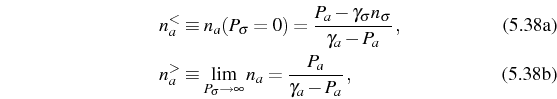
As an overall representation of the typical systems that arise in real and desired experiments, we consider three configurations, shown in Fig. (5.13), scattered in order to give a rough representative picture of the overall possibilities, around parameters estimated by Khitrova et al. (2006). Point 1 corresponds to the best system of our selection, in the sense that its decay rates are very small ( $\gamma_a=g/10$ , $\gamma_\sigma=g/100$ ), and the quantum (Hamiltonian) dynamics dominates largely the system. It is a system still outside of the experimental reach. Point 3 on the other hand corresponds to a cavity with important dissipations, that, following our analysis below, precludes the observation of any neat structure attributable to the underlying Fermi statistics. According to numerical fitting of the experiment, real structures might even be suffering higher dissipation rates (see Sec. 3.5). Point 2 represents other lead systems of the SC physics, that we will show can presents strong departure from the linear regime, in particular conditions that we will emphasize. The best semiconductor system from Fig. 5.13 is realized with microdisks, thanks to the exceedingly good cavity factors. We shall not enter into specific discussion of the advantages and inconvenient of the respective realizations and the accuracy of these estimations. From now on, we shall refer to this set of parameters as that of ``reference points'', keeping in mind that points 1 and 2 in particular represent systems that we will refer to as a ``good system'' and a ``more realistic system'', respectively.

In Fig. 5.14, the three observable of main interest for a physical understanding of the system that we have just discussed--, $n_\sigma$ and $g^{(2)}$ --are obtained numerically for the three reference points. Electronic pumping is varied from, for all practical purposes, vanishing ( $10^{-3}g$ ) to infinite () values. Various cavity pumpings are investigated and represented by the color code from no-cavity pumping (dark blue) to high, near diverging, cavity pumping (red), through the color spectrum. We checked numerically that these results satisfy Eq. (5.36). The overall behavior is mainly known, for instance the characteristic increase till a maximum and subsequent decrease of with $P_\sigma$ has been predicted in a system of QD coupled to a microsphere by Benson & (1999). This phenomenon of so-called self-quenching is due to the excitation impairing the coherent coupling of the dot with the cavity: bringing in an exciton too early disrupts the interaction between the exciton-photon pair formed from the previous exciton. Therefore the pumping rate should not overcome significantly the coherent dynamics. Too high electronic pumping forces the QD to remain in its excited state and thereby prevents it from populating the cavity. In this case the cavity population returns to zero while the exciton population (or probability for the QD to be excited) is forced to one. This effect appeared as well in the two 2LSs, with the quenching of the direct emission when the dots saturated with the excitonic pump. The cavity pumping brings an interesting extension to this mechanism. First there is no quenching for the pumping of bosons that, on the contrary, have a natural tendency to accumulate and lead to a divergence. Therefore the limiting values for when $P_\sigma\rightarrow0$ or $P_\sigma\rightarrow\infty$ are not zero, as in the previously reported self-quenching scenario. They also happen to be different:

$\begin{subequations}\begin{align}n_a^<&\equiv n_a(P_\sigma=0)=\frac{P_a-\gamma_\... ...a\rightarrow\infty}n_a=\frac{P_a}{\gamma_a-P_a}\,, \end{align}\end{subequations}$

and therefore satisfy

. Eq. (5.40b) follows from the decoupled thermal values for the populations, $n_\sigma\rightarrow P_\sigma/(P_\sigma+\gamma_\sigma)$ , and corresponds to a passive cavity where the quenched dot does not contribute at all. In this case, the emission spectrum of the system is expected to converge to

$\displaystyle S_a(\omega)=\frac1\pi\frac{\Gamma_a/2}{(\omega-\omega_a)^2+(\Gamma_a/2)^2}\,,$

(5.40)

for the cavity, and $S_\sigma(\omega)=0$ for the dot. The other limit when $P_\sigma=0$ , shows the deleterious effect of the dot on cavity population. The dot fully enters the dynamics contrary to the quenched case where it is subtracted from it.

In the works of Mu & (1992), Ginzel et al. (1993), Jones et al. (1999), Karlovich & (2001) or Kozlovskii & (1999), important application of SC for single-atom lasing were found for good cavities 1 and 2, where the coupling $g\gg\gamma_a,\gamma_b$ is strong enough. Lasing can occur when the pumping is also large enough to overcome the total losses, $P_\sigma\gg\gamma_a,\gamma_\sigma$ . Setting , $\gamma_\sigma=0$ , Eqs. (5.13) can be approximately reduced to one for the total photonic probability $\mathrm{p}[n]$ , as it has been shown by Scully & Zubairy (2002) or Benson & (1999):

$\displaystyle \frac{d\mathrm{p}[n]}{dt}=\gamma_a(n+1)\mathrm{p}[n+1]-\Big(\gamm... ...\mathrm{p}[n]+\frac{l_\mathrm{G}n}{1+l_\mathrm{S}/l_\mathrm{G}n}\mathrm{p}[n-1]$

(5.41)

The parameters that characterize the laser are the gain $l_\mathrm{G}=4g^2/P_\sigma$ and the self saturation $l_\mathrm{S}=8g^2l_G/P_\sigma^2$ . Far above threshold ( $n_al_\mathrm{S}/l_\mathrm{G}\gg1$ ), the statistics are Poissonian, $g^{(2)}=1$ , with a large intensity in the emission, $n_a=P_\sigma/(2\gamma_a)$ , and half filling of the dot, $n_\sigma=0.5$ . However, this analytic limit from the standard laser theory is not able to reproduce the self-quenching effect induced by the incoherent pump, nor the subpoissonian region ( $g^{(2)}<1$ ) where quantum effects are prone to appear. The validity of the laser theory is restricted to the narrow region, $\gamma_a\ll P_\sigma\ll \gamma_\sigma^\mathrm{P}$ , where $\gamma_\sigma^\mathrm{P}=4g^2/\gamma_a$ is the boundary for the self-quenching. In the weak coupling regime, $\gamma_\sigma^\mathrm{P}$ is the well known Purcell enhanced spontaneous decay rate of an exciton through the cavity mode. In the strongly coupled system, it can be similarly understood as the rate at which an exciton transforms into a photon. If the excitons are injected at a higher rate, there is no time for such a coherent exchange to take place and populate the cavity with photons. Fig. 5.14 shows that lasing can be achieved with system 1 in the corresponding region of pump. Here, we will solve the system exactly, covering this regime and all the other possible ones with the full quantum equations of motion.

The effect of cavity pumping depends strongly on the experimental situation. In the case of an exceedingly good system, has little effect as soon as the exciton pumping is important, $P_\sigma>\gamma_a$ . Cavity pumping becomes important again in a system like 2, where it enhances significantly the output power, with the price of superpoissonian statistics ( $g^{(2)}>1$ ). With a poorer system like point 3, some lasing effect can be found with the aid of the cavity pump: there is a nonlinear increase of and $g^{(2)}$ approaches 1 for $g<P_\sigma<10g$ . However, the weaker the coupling, the weaker this effect until it disappears completely for decay rates outside the range plotted in Fig. 5.13. In all cases, the self-quenching leads finally to a thermal mixture of photons ( $g^{(2)}=2$ ) and WC at large pumping.