

Next: SE analytical spectrum Up: The anharmonic oscillator Previous: The anharmonic oscillator Contents
First order correlation function and power spectrum
The set of operators that are needed to compute the correlator of
interest, namely
![]() , are the most general set
, are the most general set
![]() , differently than for the harmonic
oscillator in Section 2.6. The regression
matrix
, differently than for the harmonic
oscillator in Section 2.6. The regression
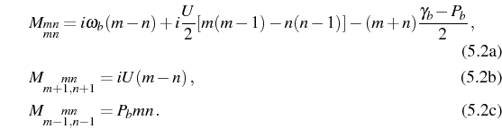
matrix ![]() is defined by the following rules:
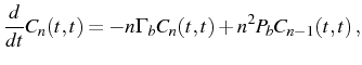
is defined by the following rules:
![\includegraphics[width=.45\linewidth]{chap5/AO/fig1-correlator.ps}](img1297.png) |
This gives rise to an infinite set of coupled equations for any
general correlator.
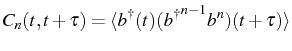
![]() is linked to all
correlators of the kind:
is linked to all
correlators of the kind:
with
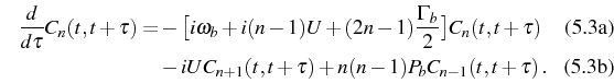
or applying again the quantum regression formula. The second set of equations,
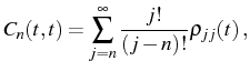
are easily solved in the two cases we are interested in. The steady state (SS) is, as we said, the thermal state [Eqs. (2.34)-(2.35)] for which
The correlators
![]() cannot be found analytically in the
general case with pump because the Hilbert space is infinite (
cannot be found analytically in the
general case with pump because the Hilbert space is infinite (
![]() ). The formula (2.105) of the
spectra must be kept in general terms for the SS emission.
). The formula (2.105) of the
spectra must be kept in general terms for the SS emission.
Subsections
Next: SE analytical spectrum Up: The anharmonic oscillator Previous: The anharmonic oscillator Contents