First order correlation function and power spectrum

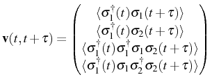
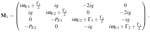
The luminescence spectrum of the system through the emission of one of the dots, $S_1(\omega)$ , requires the correlator $\langle\ud{\sigma_1}(t)\sigma_1(t+\tau)\rangle$ in Eq. (2.75). Let us write the quantum regression formula for the most general set of operators $\{C_{\{m,n,\mu,\nu\}}=\ud{\sigma}_1^m\sigma_1^n\ud{\sigma}_2^\mu\sigma_2^\nu\}$ , with , , $\mu$ , $\nu\in\{0,1 \}$ . The regression matrix is defined by:

$\begin{subequations}\begin{align}&M_{\substack{mn\mu\nu\\ mn\mu\nu}}=i\omega_{E1... ...u\nu\\ m,1-n,\mu,1-\nu}}=-ig[n(1-\nu)+\nu(1-n)]\,, \end{align}\end{subequations}$

and zero everywhere else.

**Figure 4.2:** Chain of correlators--indexed by $\{\eta\}=(m,n,\mu,\nu)$ --linked by the Hamiltonian dynamics with pump and decay for two coupled 2LS. On the left (resp., right), the set $\bigcup_k\mathcal{N}_k$ (resp., $\bigcup_k\tilde{\mathcal{N}}_k$ ) involved in the equations of the two-time (resp., single-time) correlators. In green are shown the first manifolds $\mathcal{N}_1$ and $\tilde{\mathcal{N}}_1$ that correspond to the LM (see Fig. 3.2), and in blue, the second manifold $\mathcal{N}_2$ and $\tilde{\mathcal{N}}_2$ . The equation of motion $\langle \ud{\sigma_1}(t)C_{\{\eta\}}(t+\tau)\rangle$ with $\eta\in\mathcal{N}_k$ requires for its initial value the correlator $\langle C_{\{\tilde\eta\}}\rangle$ with $\{\tilde\eta\}\in\tilde{\mathcal{N}}_k$ defined from $\{\eta\}=(m,n,\mu,\nu)$ by $\{\tilde\eta\}=(m+1,n,\mu,\nu)$ , as seen on the diagram. The thick red arrows indicate which elements are linked by the coherent (SC) dynamics, through the coupling strenght , while the green/blue thin arrows show the connections due to the incoherent QD pumpings. The sense of the arrows indicates which element is ``calling'' which in its equations. The self-coupling of each node to itself is not shown. This is where $\omega_{E1,E2}$ and $\Gamma_{1,2}$ enter. These links are obtained from the rules in Eqs. (4.4), that result in the matrices $\mathbf{M}_1$ and $\mathbf{M}_0$ . The number of correlators needed to compute the spectrum is truncated naturally (with four elements) thanks to the saturation of the 2LSs.
$\includegraphics[width=0.8\linewidth]{chap4/manifolds/Fig6.ps}$

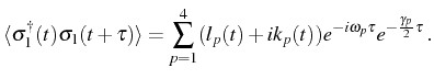
For the computation of the spectrum, we need two more correlators and equations than in the two coupled HOs (see Fig. 3.2). In Fig. 4.2 we can see a schema of this finite set of correlators (left) and mean values (right), labelled with the indices $\{\eta\}=\{m,n,\mu,\nu\}$ . The coherent (through ) and incoherent (through $P_{E1,E2}$ ) links between the various correlators, given by the regression matrix, are shown with arrows (see a detailed explanation of the figure in the caption). Thanks to the saturation of both modes, being 2LSs, we obtain a simple equation,

$\displaystyle \partial_\tau\mathbf{v}(t,t+\tau)=-\mathbf{M}_1\mathbf{v}(t,t+\tau)\,,$

(4.5)

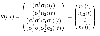
for the correlators

$\displaystyle \mathbf{v}(t,t+\tau)= \begin{pmatrix}\langle\ud{\sigma_1}(t)\sigm... ...angle\ud{\sigma_1}(t)\sigma_1\ud{\sigma_2}\sigma_2(t+\tau)\rangle \end{pmatrix}$

(4.6)

with the matrix

$\displaystyle \mathbf{M}_1= \begin{pmatrix}i\omega_{E1}+\frac{\Gamma_1}{2} & ig... ...}&-ig\\ -P_{E2}&0&-ig&i\omega_{E1}+\Gamma_2+\frac{\Gamma_1}{2} \end{pmatrix}\,.$

(4.7)

At low excitation, this system is reduced to the LM, where only the first two correlators and columns/rows of $\mathbf{M}_1$ remain. The general solution (for positive $\tau$ ), $\mathbf{v}(t,t+\tau)=e^{-\mathbf{M}_1\tau}\mathbf{v}(t,t)$ , leads to a correlator of the form:

$\displaystyle \langle\ud{\sigma_1}(t){\sigma_1}(t+\tau)\rangle=\sum_{p=1}^4 (l_p(t)+i k_p(t)) e^{-i\omega_p\tau}e^{-\frac{\gamma_p}{2}\tau}\,.$

(4.8)

The coefficients

and

depend on the dynamics of the mean values,

$\displaystyle \mathbf{v}(t,t)= \begin{pmatrix}\langle\ud{\sigma_1}\sigma_1\rang... ...rix} = \begin{pmatrix}n_1(t)\\ n_{12}(t)\\ 0\\ n_\mathrm{B}(t) \end{pmatrix}\,.$

(4.9)

Here, we have introduced some notation in order to highlight the meaning of each quantity: $n_i=\langle\ud{\sigma_i}\sigma_i\rangle\in\mathbb{R}$ (for

) are the probabilities of having each dot excited (1 or 2), independently of the other dot's state. $n_B\in\mathbb{R}$ is the joint probability that both dots are excited:

$\displaystyle n_B=\langle\ud{\sigma_1}\sigma_1\ud{\sigma_2}\sigma_2\rangle\,.$

(4.10)

If the QDs were uncoupled, we would have

. The quantity $n_{12}\in\mathbb{C}$ is the coherence between the dots due to the direct coupling. The third mean value of vector $\mathbf{v}$ , $\langle\ud{\sigma_1}\ud{\sigma_1}\sigma_1\sigma_2\rangle$ , is zero due to the fact that each dot can only host one exciton at a time and, therefore, $\ud{\sigma_1}\ud{\sigma_1}=0$ . This simplifies the algebra as only three elements of the first row in matrix $e^{-\mathbf{M}_1\tau}$ need to be computed in order to obtain the correlator of Eq. (4.8).

Note that is also the population of state $\ket{B}$ (see Fig. 4.1). The population of the intermediate state $\ket{Ei}$ , and also the probabilities of having only dot excited, is given by $n_{Ei}=n_i-n_B$ . The population of the ground state is given by $n_{G}=1-n_1-n_2+2n_B$ . The last interesting averages are the excitation of each dot, or , and the total excitation in the system, .

In order to insert these average quantities in the expression for the spectrum, they must be either time integrated in the SE case to give $\mathbf{v}^\mathrm{SE}=\int_0^\infty \mathbf{v}(t,t)dt$ (and the coefficients $l_p^\mathrm{SE},k_p^\mathrm{SE}$ ) or computed directly in the SS to give $\mathbf{v}^\mathrm{SS}=\lim_{t\rightarrow\infty} \mathbf{v}(t,t)$ (and the coefficients $l_p^\mathrm{SS},k_p^\mathrm{SS}$ ). The normalized spectra for the direct emission of dot follows from our general expression as:

$\displaystyle S_1(\omega)=\frac1{\pi}\sum_{p=1}^4\left[L_p\frac{\frac{\gamma_p}... ...{\omega-\omega_p}{\big(\frac{\gamma_p}{2}\big)^2+(\omega-\omega_p)^2}\right]\,,$

(4.11)

with

being the normalized coefficients in the SE or SS case.

Subsections