

The harmonic oscillator: bosonic states
The quantum harmonic oscillator (HO) is the most natural
description for field excitations. Basically, it consists in the
endless possibility to create particles through a creation (or ladder)
operator ![]() . It is then the perfect match for
bosons. Bosons are particles, quasi-particles or composite
particles that have an integer total spin and can be many to occupy
the same state. The electromagnetic field, composed of photons, is
exactly modelled by HOs. Also, matter excitations, such as excitons in
semiconductors, that are composite bosons in the
regime2.1
. It is then the perfect match for
bosons. Bosons are particles, quasi-particles or composite
particles that have an integer total spin and can be many to occupy
the same state. The electromagnetic field, composed of photons, is
exactly modelled by HOs. Also, matter excitations, such as excitons in
semiconductors, that are composite bosons in the
regime2.1
![]() , can be well represented in this basic
picture, since when the density is very low, their energy levels are
far from saturated and the Pauli effects arising from the fermionic
components (electrons and holes) are negligible. We will see in
Sec. 2.2 how to deal with matter
excitations when fermionic effects are important.
, can be well represented in this basic
picture, since when the density is very low, their energy levels are
far from saturated and the Pauli effects arising from the fermionic
components (electrons and holes) are negligible. We will see in
Sec. 2.2 how to deal with matter
excitations when fermionic effects are important.
Let us now go quickly through the basic properties of the HO and its
possible realizations. To begin with, a state with one particle is
simply defined as the application of a creation operator ![]() on
the vacuum,
on
the vacuum,
![]() . The
. The ![]() -particle state is
obtained through recursive creations:
-particle state is
obtained through recursive creations:
with a normalization prefactor
With such properties,
where
In order to further investigate interesting states of the HO, one can
imagine an ideal detector that absorbs field particles of all
frequencies one by one. A ``detection'' means removing one particle
from the initial field state ![]() to get the final state
to get the final state
![]() . As described by Glauber (1963b), the probability
per unit time to detect a particle whatever the final state,
. As described by Glauber (1963b), the probability
per unit time to detect a particle whatever the final state,
![]() , is given by
, is given by
which is equal to the mean number of particles,2.2
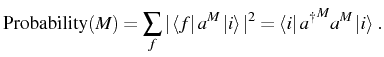
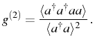
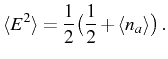
Here, we see the importance of normal order and how it is linked to observable quantities in photon counting experiments. The most celebrated of those is the two-particle coincidence experiment developed by Hanbury Brown (1956) with photons. Taken at zero delay (we will see more general two-time expressions in Sec. 2.7), the probability of detecting two photons informs about the statistics of the particle number distribution, which is an important property of the quantum state of the field. A widely used quantity is the degree of second-order coherence (or, equivalently, second-order correlation function at zero delay)
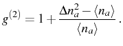
It is linked to the variance (or second cumulant)
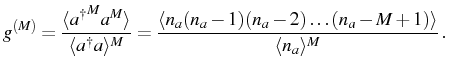
More generally, the degree of Mth-order coherence reads:
The number state or Fock state that we already
introduced, has zero variance around the mean number of particles ![]() ,
that is completely determined. This results in
,
that is completely determined. This results in
![]() --which
jumps from 0 at
--which
jumps from 0 at ![]() to
to ![]() at
at ![]() , as it corresponds to a
two-photon observable. It is always below
, as it corresponds to a
two-photon observable. It is always below ![]() . This feature of
. This feature of
![]() is associated to some kind of quantum behavior.
is associated to some kind of quantum behavior. ![]() is a very ``quantum'' state, in the sense that each quantum counts:
the change in number has some strong impact. This is in contrast with
a classical continuous field where a photon would be an infinitesimal
contribution, which removal or addition has no effect whatsoever, as
we shall see shortly.
is a very ``quantum'' state, in the sense that each quantum counts:
the change in number has some strong impact. This is in contrast with
a classical continuous field where a photon would be an infinitesimal
contribution, which removal or addition has no effect whatsoever, as
we shall see shortly.
If one photon is detected from an initial state
![]() , no
second photon can be expected as it gets projected into vacuum
, no
second photon can be expected as it gets projected into vacuum
![]() when measuring the first photon. For the number
states, the probability of emission decreases as photons get
detected. At high numbers, one particle more or one particle less does
not make much difference (
when measuring the first photon. For the number
states, the probability of emission decreases as photons get
detected. At high numbers, one particle more or one particle less does
not make much difference (
![]() ). A classical description
and understanding of the state starts to be valid at this point and
). A classical description
and understanding of the state starts to be valid at this point and
![]() tends to
tends to ![]() . Similar behavior is found for higher orders of
coherence:
. Similar behavior is found for higher orders of
coherence:
The probability of having
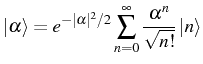
Another interesting state is the coherent state
![]() ,
derived by Schrödinger for the first time in 1926 but fully
developed in its quantum optical context by
Glauber (1963a). It is characterized by being the eigenstate
of the destruction operator:
,
derived by Schrödinger for the first time in 1926 but fully
developed in its quantum optical context by
Glauber (1963a). It is characterized by being the eigenstate
of the destruction operator:
with eigenvalue a complex number,
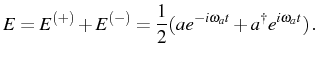
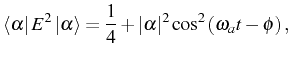
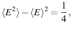
This can be also considered the expression a general bosonic field. In a coherent state, the expectation value of the electric field, the intensity operator and the field variance, respectively, are given by
which basically means that the quantum fluctuations of the field

having no electric mean field but quantum fluctuations.
For a coherent state, the variance of the particle number distribution is the same as the mean number
In fact, all cumulants of the distribution converge to this value and the state is coherent at all orders (in Glauber's sense):
and analyzing the particle number distribution
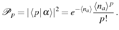
This is a Poissonian distribution.2.3 A distribution with
States like ![]() and
and
![]() that are completely described
with a wavefunction (one ket) are known as pure states. They
can be a good description for a field in some limiting cases where it
is very well isolated from the environment, and it experiences only
coherent dynamics given by a Hamiltonian. For example, the
evolution of
that are completely described
with a wavefunction (one ket) are known as pure states. They
can be a good description for a field in some limiting cases where it
is very well isolated from the environment, and it experiences only
coherent dynamics given by a Hamiltonian. For example, the
evolution of
![]() through the free
Hamiltonian (2.3) (a phase rotation in its
complex parameter) remains always perfectly determined by a
wavefunction,
through the free
Hamiltonian (2.3) (a phase rotation in its
complex parameter) remains always perfectly determined by a
wavefunction,
![]() . However, in general, one
should consider the contamination of this dynamics due to the field
being irremediably in contact with the exterior world. In principle
one could model all possible interactions with the environment with a
more comprehensive Hamiltonian that includes all the processes that
affect the field
. However, in general, one
should consider the contamination of this dynamics due to the field
being irremediably in contact with the exterior world. In principle
one could model all possible interactions with the environment with a
more comprehensive Hamiltonian that includes all the processes that
affect the field ![]() . This is, of course, an impossible task if one
takes it seriously (having to model the whole universe!), and quite a
difficult one even with drastic approximations. One cannot and does
not want to keep track of all the degrees of freedom affecting the
field. This lack of interest on the external world results in
decoherence for our system.
. This is, of course, an impossible task if one
takes it seriously (having to model the whole universe!), and quite a
difficult one even with drastic approximations. One cannot and does
not want to keep track of all the degrees of freedom affecting the
field. This lack of interest on the external world results in
decoherence for our system.
In the previous example of the evolution of a coherent state, one can
imagine that the field ![]() is affected by an incoherent process
that interrupts its coherent free evolution (like a measurement that
randomizes its phase). We are not interested in this process by itself
and therefore only retain its effect on our field: the rate at which
the perturbation happens. After some time
is affected by an incoherent process
that interrupts its coherent free evolution (like a measurement that
randomizes its phase). We are not interested in this process by itself
and therefore only retain its effect on our field: the rate at which
the perturbation happens. After some time ![]() , when the probability
that a first event has happened is
, when the probability
that a first event has happened is
![]() , we cannot say
anymore that the state of the system is defined by
, we cannot say
anymore that the state of the system is defined by
![]() . We only know that this is so with a probability
. We only know that this is so with a probability
![]() and that the state of the system is
and that the state of the system is
![]() with a probability
with a probability
![]() . Therefore we need a mixture
of two wavefunctions, rather than only one like for the pure
state. Following this idea, the dynamics of the system can be
understood as a succession of coherent periods and incoherent random
(from our ignorant point of view) events that project the wavefunction
into a given state. Those are the so-called quantum jumps. One
can guess that after some time and a complicated mixture of
quantum trajectories, we loose track completely of the phase of
the state. This means that the steady state (SS) of this system is
expected to be a mixture of coherent states where all possible phases
have the same probability,
. Therefore we need a mixture
of two wavefunctions, rather than only one like for the pure
state. Following this idea, the dynamics of the system can be
understood as a succession of coherent periods and incoherent random
(from our ignorant point of view) events that project the wavefunction
into a given state. Those are the so-called quantum jumps. One
can guess that after some time and a complicated mixture of
quantum trajectories, we loose track completely of the phase of
the state. This means that the steady state (SS) of this system is
expected to be a mixture of coherent states where all possible phases
have the same probability,
![]() .
.
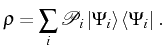
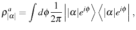
A consistent way to express this situation, and the most general
description of the state of the system, is using the density
matrix operator ![]() . In general, the density matrix can always
be put in its diagonal form, as a linear superposition of
projectors,2.4
. In general, the density matrix can always
be put in its diagonal form, as a linear superposition of
projectors,2.4
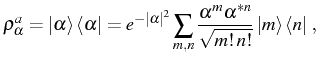
has all off-diagonal terms in the number state basis. On the other hand, in our previous example of a mixture of coherent states with a random phase, the SS density matrix can be constructed as
from which follows that
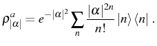
In each basis we can see two aspects of the decoherence that the coherent state of Eq. (2.23) has suffered. In the first one, the most direct consequence of the phase randomization manifests in the lack of off-diagonal elements between states with different phases. The second basis of number states evidences that the particle number distribution is still Poissonian but also that the off-diagonal elements between number states have been washed out. As it is the case for any mixture diagonal in the number state basis, the average of the field is zero,
These results are closer to those of a number state (2.16) than of a coherent state (2.13). However, the state is still coherent at all orders.
The next important state to discuss is the thermal mixture. It
is the state whose bosonic excitations, the particles of the field,
are thermally spread among the energy levels. We will see in
Sec. 2.4 that this is the result of the
interaction with a reservoir of particles at a given temperature
![]() . The density matrix for a given mode
. The density matrix for a given mode ![]() can be derived
from the Bose-Einstein statistics as
can be derived
from the Bose-Einstein statistics as
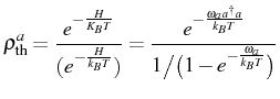
where
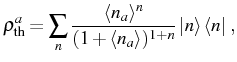
with the average occupation being the Bose-Einstein distribution,
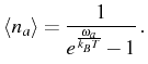
This formula was guessed by M. Planck in 1900 to fit the experiments on blackbody radiation and later derived by Bose from a statistical arguments for photons: Bose merely required that the particles be indistinguishable. As the system is in thermal equilibrium with a bosonic bath, their average occupation at the frequency
Let us analyze the process that leads to the thermal equilibrium. We
suppose that the reservoir population is not influenced by the
interaction with our system (approximation discussed in
Sec. 2.4). The system does evolve from
vacuum into the SS of thermal equilibrium and the mean value depends
on time
![]() . The total rate of incoming particles from the
reservoir to the system is given by
. The total rate of incoming particles from the
reservoir to the system is given by
![]() . The effective rate of excitation to the system
(analogue for bosons of the Einstein B-coefficient), is
. The effective rate of excitation to the system
(analogue for bosons of the Einstein B-coefficient), is
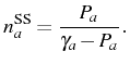
It vanishes at
The new parameter
![$\displaystyle \frac{d \langle n_a(t)\rangle }{dt}=-\gamma_a\langle n_a(t)\rangle +P_a[1+\langle n_a(t)\rangle ]$](img212.png)
and leads in the SS to Eq. (2.30), now
At very high temperatures, as the effective income of particles approaches the outcome,
Logically, given its origin, the thermal state does not exhibit any coherence properties at any order (other than the first for a single mode2.5),
and in particular
that exceed those of the Poissonian distribution by
In the following chapters and sections, we will study different configurations and processes which generate the states that we just described. Very rarely, the state of the system is completely thermal, or coherent, or has a purely Poissonian statistics. In most of the cases, the bosonic field (of light or matter) is a convolution of different states. For example, a cothermal state, the superposition of a coherent and a thermal state, first explored by Lachs (1965), has a distribution of particles
![$\displaystyle \bra{n}\rho^a_\mathrm{coth}\ket{n}=\mathcal{P}_\mathrm{coth}(n)=e...
...}{(1+n_\mathrm{t})^{n+1}}L_n[-\frac{n_\mathrm{c}/n_\mathrm{t}}{1+n_\mathrm{t}}]$](img225.png)
where
The density matrix of the optical field assumes a transparent expression in the
Cothermal states represent a simple but precise description of a
system where coherent and incoherent processes compete. For instance,
this is the case of Bose-Einstein condensation in the presence of
decoherence, as it was shown in Ref. 16 of
the list of my publications ![[*]](crossref.png) .
.
Elena del Valle ©2009-2010-2011-2012.