Vanishing pump (and SE) case in the manifold picture

Only in the case of vanishing pump, that corresponds as well to the SE situation, the simple SC/WC classification holds. In this limit, we recover the familiar expression for the half Rabi frequency,

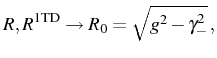
$\displaystyle R,R^\mathrm{1TD}\rightarrow R_0=\sqrt{g^2-\gamma_-^2}\,,$

(4.26)

as in Eq. (3.33). The parameters simplify to $z_{1,2}\rightarrow\sqrt{(R_0\pm i\gamma_+)^2}$ and the associated condition for SC reduces to

being real, or more explicitly $g>\vert\gamma_-\vert$ , as in the LM. In SC the positions and broadenings of the four peaks reduce to

$\begin{subequations}\begin{align}&\frac{\gamma_1}{2}+i\omega_1=\gamma_++iR_0\,,\... ...quad&\frac{\gamma_4}{2}+i\omega_4=\gamma_+-iR_0\,. \end{align}\end{subequations}$

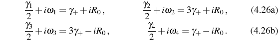
The two pairs of peaks

and

sit on the same points although they have different broadenings. This means that all peaks undergo the transition into WC simultaneously, when $R_0\rightarrow i\vert R_0\vert$ and both $z_{1,2}\rightarrow\vert\gamma_+\pm\vert R_0\vert\vert i$ become imaginary, giving

$\begin{subequations}\begin{align}&\omega_p=0\,,\quad p=1,2,3,4\,,\\ &\frac{\gamm... ...quad\frac{\gamma_4}{2}=3\gamma_++\vert R_0\vert\,, \end{align}\end{subequations}$

since $\gamma_+>\vert R_0\vert$ in WC regime. The four peaks collapse into four Lorentzians at the origin with four different broadenings. The transition $SC\rightarrow WC$ is not smooth in its description, in the sense that, for instance, peak 2 takes the place of 4 (as well, 4 of 3 and 3 of 2 as we show below). But this is simply a sign that the dressed states disappear in WC. In any case, all observables behave completely smoothly (as in the LM).

It it important to note that, as a result of the two pairs of peaks sitting always on the same two frequencies, the final spectra can only be either a single peak or a doublet, both shapes being possible in SC or WC regimes (as in the LM and for the same reasons).

The manifold picture (see Section 2.5.2) gives a very intuitive derivation and interpretation of the results in this limit. We consider the nonhermitian Hamiltonian $H_\mathrm{n.h.}$ that results from making the substitution $\omega_{E1,E2}\rightarrow\omega_{E1,E2}-i\gamma_{E1,E2}/2$ in Eq. (4.1), in order to include the decay of the modes. Diagonalizing the Hamiltonian in the first manifold [as with the two HOs, see Eq. (2.56) and discussions related in Chapter 3], we obtain

$\displaystyle H_\mathrm{n.h.}=E_\mathrm{G}\ket{G}\bra{G}+E_\mathrm{U}\ket{U}\bra{U}+E_\mathrm{L}\ket{L}\bra{L}+E_\mathrm{B}\ket{B}\bra{B}$

(4.29)

with dressed complex energies

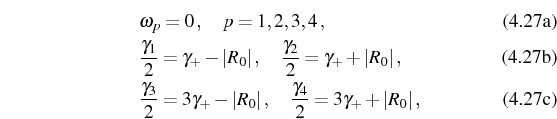
$\displaystyle E_\mathrm{G}=0\,,\quad E_{\substack{\mathrm{U}\\ \mathrm{L}}}=\om... ...\pm R_0\,,\quad E_\mathrm{B}=2\omega_{E1}-i\frac{\gamma_{E1}+\gamma_{E2}}{2}\,.$

(4.30)

Applying Eq. (2.96) between the energies in Eq. (4.30), leads to the positions and broadenings of Eq. (4.27)-(4.28) in the way that we now explain. In Fig. 4.1(a) we can see the four possible transitions in the manifold picture: one can check that

$\bullet$: the lower transitions (in blue), from $\ket{U}$ and $\ket{L}$ , coincide, respectively, with the expressions for peaks 1 and 4 in SC, Eq. (4.27) and 1 and 2 in WC, Eq. (4.28);
$\bullet$: the upper transitions (in red), towards $\ket{L}$ and $\ket{U}$ , coincide with the expressions for peaks 2 and 3 in SC, Eq. (4.27) and 3 and 4 in WC, Eq. (4.28).

The upper transitions have a larger broadening than the lower due to the addition of the uncertainties in energy of the levels involved, brought by the spontaneous decay. This is also the case in the LM, if we consider the individual transitions, in terms of the states inside each manifold. But, in the end, the resulting SE from an initial state takes place, not only at the same two energies, but also with the same broadenings, regardless of the starting manifold. The spectral shape (the Rabi doublet) is manifold independent. The inhomogeneity in the broadenings for coupled QDs, makes a difference in the SE spectra out of the linear regime (with manifolds

involved). The spectra, like the populations, is different in both models if the initial state is that of the second manifold, $\ket{B}$ (or $\ket{1,1}$ ), because in the LM there are two more states in the same manifold to couple with, than for the 2LSs.

On the other hand, the SS case in the limit of vanishing pump is exactly the linear regime, where only the vacuum and first manifold are populated. The spectra in this limit converge with the LM and also it can be analyzed in terms of manifolds by extension. For instance, the spectrum in Fig. (4.3) corresponds to SC for vanishing pump, for $\gamma_{E1}=g$ and $\gamma_{E2}=g/2$ . The lower transition peaks, in blue, dominate over the broader and weak upper peaks, in red, and as a result, the splitting in dressed modes is visible in the observed spectrum, in black. We now use this configuration in what follows to explore the effect of the incoherent continuous pump.