Coherent coupling

Coherent processes are those that can be written as a Hamiltonian (always hermitian) and included in the Schrödinger equation:

$\displaystyle \frac{d\rho}{dt}=i[\rho,H]\,.$

(2.53)

We already wrote the free evolution of the bosonic and fermionic fields in Eq. (2.3) and (2.47). Two fields

and

in the same point of space can interact linearly with a Hamiltonian that is of the form

$\displaystyle H_{ab}=g(a\ud{b}+\ud{a}b)\,.$

(2.54)

If the detuning between the modes,

$\displaystyle \Delta=\omega_a-\omega_b\,,$

(2.55)

is small as compared to the coupling, during the dynamics of $H_{ab}$ , an

-particle becomes

and vice-versa. The frequencies are assumed much larger than the coupling and detuning between the modes, $\omega_{a,b}\ll g,\Delta$ , so that the Rotating Wave Approximation^2.10 holds. The Hamiltonian $H=H_a+H_b+H_{ab}$ does not conserve the number of particles

and

separately, as they experience a mutual conversion in the form of Rabi oscillations. The particles whose number is conserved are the eigenstates of

. But in order to diagonalize

we must specify the nature of the fields.

In this text, field will be always the electromagnetic field inside a cavity, where one mode with frequency $\omega_a$ is selected. Depending on the model for the material excitation, is described by, typically, another HO, giving rise to the linear model (LM) developed by Hopfield (1958), or by a 2LS, giving rise to the Jaynes & Cummings (1963) model (JCM), discussed in the Introduction. Those are the most fundamental cases as they describe material fields with Bose and Fermi statistics, respectively. Possible extensions are a collection of HOs; this has been considered by Rudin & Reinecke (1999) and more recently by Averkiev et al. (2009), or of many 2LS like in the work of Dicke (1954), or a three-level system as considered by Bienert et al. (2004), etc...

The parameter depends on both the properties of the cavity and the emitters: $g\sim \sqrt{f_b/V_a}$ , where is the effective cavity volume and the oscillator strength of the emitter. Therefore, in order to achieve strong coupling experimentally, the cavity must have a high quality factor ( $\gamma_a\sim \omega_a/Q_a$ ) and a small effective volume . The emitters must be placed close to the anti-node of the electric field in the cavity, have transition frequencies close to resonance with the cavity mode and exhibit high oscillator strengths.

The linear model (discussed in Chapter 3) corresponds to the coupling of two bosonic modes, and . The Hamiltonian can be straightforwardly diagonalized, giving:

$\begin{subequations}\begin{align}H=\omega_\mathrm{U}\ud{u}u+\omega_\mathrm{L}\ud... ...athcal{R}=\sqrt{g^2+\big(\frac{\Delta}2\big)^2}\,, \end{align}\end{subequations}$

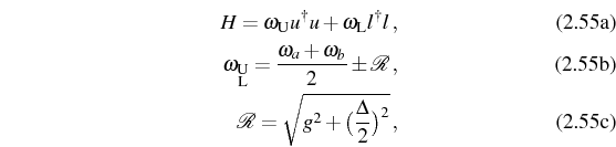
with new Bose operators $u=\cos\theta \, a+\sin\theta \, b$ and $l=-\sin\theta \, a+\cos\theta \, b$ , determined by the mixing angle,

$\displaystyle \theta=\arctan{\Big(\frac{g}{\frac\Delta2+\mathcal{R}}\Big)}\,.$

(2.57)

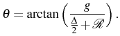
These new modes are the polaritons (or dressed states) with $\mid\mid 1,0\rangle\rangle =\ud{u}\ket{\mathrm{0}}$ and $\mid\mid 0,1\rangle\rangle =\ud{l}\ket{\mathrm{0}}$ , where $\ket{\mathrm{0}}$ is the vacuum, $\ket{m,n}$ is the Fock state of in the bare basis and $\mid\mid m,n\rangle\rangle$ the Fock state in the dressed basis.

**Figure 2.1:** Solid black: Bare energies of the cavity photon (horizontal line) and of the exciton (tilted) as a function of detuning $\Delta=\omega_a-\omega_b$ . Dashed black: Eigenenergies of the total system Hamiltonian, without dissipation nor pumping [Eq. (2.56a)]. The exciton-like state at large negative $\Delta$ has become a photon-like state at large positive $\Delta$ , and vice-versa. Around $\Delta=0$ , both modes are an admixture of exciton and photon.
$\includegraphics[width=.5\linewidth]{chap2/Case-(c)-Pb_0.15--Splitting-with-det.eps}$

The energies defined by Eq. (2.56b) are displayed in Fig. 2.1 with dashed lines, on top of that of the bare modes, with thick lines, as detuning is varied by changing the energy of the emitter and keeping that of the cavity constant. The anticrossing always keeps the upper mode U higher in energy than the lower L one, strongly admixing the light and matter character of both particles. If the system is initially prepared as a bare state--which is the natural picture when reaching the SC from the excited state of an emitter--the dynamics is that of an oscillatory transfer of energy between light and matter. In an empty cavity, the time evolution of the probability to have an exciton when there was one at , is given by:

$\displaystyle \mathcal{P}_\mathrm{exc}=\vert\bra{0,1}e^{-iHt}\ket{0,1}\vert^2=\sin^4\theta+\cos^4\theta+2\sin^2\theta \cos^2\theta\cos(2\mathcal{R}t)\,,$

(2.58)

which results in oscillations between the bare modes at the so-called Rabi frequency, given by $2\mathcal{R}$ . At resonance, these oscillations reach their maximal amplitude $\mathcal{P}_\mathrm{exc}=\cos^2(\mathcal{R}t)$ , making possible a complete photon conversion. In this text, we will refer to $\mathcal{R}$ directly as the Rabi frequency for simplicity, keeping in mind that there is a factor

that links it to the oscillations.

On the other hand, when the coupled modes are far from resonance $\Delta\gg g$ , they affect perturbatively each other as we can see in Fig. 2.1. In this regime, the small difference in energy between the coupled and bare modes is known as the Stark shift. The Rabi frequency, when $g/\Delta\rightarrow 0$ is $\mathcal{R}\rightarrow \vert\Delta\vert/2+g^2/\vert\Delta\vert$ so that the Stark shift of each mode amounts to the same quantity

$\displaystyle s_{\substack{a\\ b}}=\pm\frac{g^2}{\Delta}\,.$

(2.59)

The second interesting possibility is when the matter field is a 2LS. We will denote it by $\sigma$ for clarity and discuss it in more details in Chapters 5 and 6. The Jaynes-Cummings Hamiltonian $H=H_a+H_\sigma+H_{a\sigma}$ can be diagonalized in a given manifold with a fixed (and integer) number of excitation $n=\langle n_a\rangle +\langle n_\sigma\rangle >0$ : $\mathcal{M}_n=\{\ket{n,0},\ket{n-1,1}\}$ . Rewriting the Hamiltonian as a sum of all manifold's contributions,

$\displaystyle H=\sum_nH_n=\sum_{n}\Big[ n\omega_a \ket{n,0}\bra{n,0}+ \Big( (n-1)\omega_a+\omega_\sigma \Big) \ket{n-1,1}\bra{n-1,1}$
$\displaystyle + g\sqrt{n} \Big( \ket{n-1,1}\bra{n,0}+ \ket{n,0}\bra{n-1,1} \Big)\Big]\,,$			(2.60)

it can be diagonalized in each subspace as

$\displaystyle H=\sum_n \Big[ \omega_\mathrm{U}^n\mid\mid 1_n,0\rangle\rangle \l... ..._\mathrm{L}^n\mid\mid 0,1_n\rangle\rangle \langle\langle 0,1_n\mid\mid \Big]\,.$

(2.61)

The eigenstates and eigenenergies are now

-dependent:

$\displaystyle \omega_{\substack{\mathrm{U}\\ \mathrm{L}}}^n=\frac{n\omega_a+\omega_\sigma}2\pm\mathcal{R}_n\,,$

(2.62)

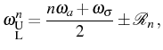
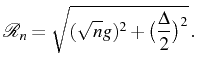
as well as the (half) Rabi frequency:

$\displaystyle \mathcal{R}_n=\sqrt{(\sqrt{n}g)^2+\big(\frac{\Delta}2\big)^2}\,.$

(2.63)

In the case of the Stark shifts, only that of the 2LS depends on the manifold:

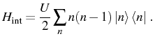
$\displaystyle \begin{eqnarray}s_a&=&\frac{g^2}{\Delta}\,,\\ s_\sigma&=&-(2n-1)\frac{g^2}{\Delta}\,. \end{eqnarray}$

(2.64a)

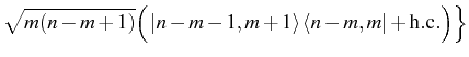
The manifold structure is the fundamental difference between the coupling of mode with a bosonic or a fermionic mode. The -manifold in the first linear case, is composed by the states $\{\ket{n-m,m}\}$ with $m=0,\hdots, n$ . The Hamiltonian can be also written in these terms, in the bare or polariton basis,

$\displaystyle H=\sum_n \Big\{$	$\displaystyle \displaystyle \sum_{m=0}^{n}$	$\displaystyle \Big[(n-m)\omega_a+m\omega_b\Big] \ket{n-m,m}\bra{n-m,m}+$
	$\displaystyle + g \displaystyle \sum_{m=0}^{n-1}$	$\displaystyle \sqrt{m(n-m+1)} \Big( \ket{n-m-1,m+1}\bra{n-m,m}+\mathrm{h.c.} \Big)\Big\}$
$\displaystyle =\sum_n$	$\displaystyle \displaystyle \sum_{p=0}^{n}$	$\displaystyle \Big[(n-p)\omega_\mathrm{U}+p\omega_\mathrm{L}\Big] \mid\mid n-p,p\rangle\rangle \langle\langle n-p,p\mid\mid \,,$	(2.65)

which makes it explicit that the energy of an excitation, $\omega_{\mathrm{U,L}}$ , is independent of the manifold. We will see in Chapter 5 that if we consider the excitonic particle-particle interactions with a Hamiltonian that carries nonlinear terms in

, such as

$\displaystyle H_\mathrm{int}=\frac{U}{2}\ud{b}\ud{b}bb=\frac{U}{2}n_b(n_b-1)\,,$

(2.66)

this indistinguishability is lost. The energy

accounts for the strength of the interactions and is positive in the case of weakly repulsive excitons. A linear simplification of the total Hamiltonian, as in Eq. (2.56a) and (2.65) is no longer possible as the eigenenergies now depend on the manifold:

$\displaystyle H_\mathrm{int}=\frac{U}{2}\sum_n n(n-1)\ket{n}\bra{n}\,.$

(2.67)

All these cases are indistinguishable when the excitation is very low and the system only probes up to the first manifold, as it is not until a second excitation arrives that interactions or fermionic effects enter the picture. It is one of the goals of this text to explore the differences arising between the different models and physical systems when .

A last interesting point to discuss is the coherent excitation of a mode via coupling to a monochromatic laser. For instance, the cavity field can be excited directly with a classical electromagnetic field $F(t)=\langle E(t)\rangle$ (in a coherent state) with frequency $\omega_\mathrm{L}$ , like that of Eq. (2.13). The corresponding Hamiltonian,

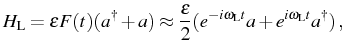
$\displaystyle H_\mathrm{L}=\epsilon F(t)(\ud{a}+a)\approx\frac{\epsilon}{2}(e^{-i\omega_\mathrm{L}t}a+e^{i\omega_\mathrm{L}t}\ud{a})\,,$

(2.68)

drives the cavity field into a coherent state. The same can happen with the excitonic field, changing

operators for the

or $\sigma$ . If the excitation intensity is strong, it may result in the appearance of new eigenstates in the system and Rabi oscillations with proportional magnitude. On the other hand, if it is weak, it can be used to probe the structure of the system without altering it, as we will see in Sec. 2.5.