First order coherence function and the power spectrum

Studying light-matter interaction in a given system, means probing the Hamiltonian structure described in Sec. 2.3. For that purpose, the manifolds need to be excited and the cavity mirrors must let particles leak out so that we can measure them. Emission (and excitation if it is incoherent) comes with the price of decoherence. This decoherence changes the underlying manifold structure (by broadening and renormalizing lines, in much the same way as described by Weisskopf).

In order to minimize the effects on decoherence and keep the SC physics as ``pure'' as possible, several experimental options are available, as explained for example by Agarwal & Puri (1986). The excitation can be of the kind of Eq. (2.68). In atomic physics, a coherent continuous wave (cw) pumping, in the form of a monochromatic laser shined on the atom, is used to probe (if weak) or drive (if strong) the system inside the cavity in the SS. In semiconductors, this excitation process corresponds to optical resonant excitation of the quantum dot or well. In this case, the direction of excitation and collection of the emission is the same. Exciting resonantly, it is difficult to distinguish the light emitted by the system from that reflected from the sample as they have similar frequencies. This is one reason why the experiments are usually done with nonresonant excitation. However, in the last few years, some experiments have been carried out where clever configurations allowed to resonantly drive a single self assembled QDs. Muller et al. (2007) used a waveguide as the excitation channel to separate it from the emitted light, reporting the first measurement of resonant fluorescence in this system.

A quantity that can be measured under the coherent cw, is the amplitude of the field scattered by the driven atom, $\langle a\rangle$ , given that the output is a coherent state of cavity photons. The intensity of the scattered field $I(\omega_\mathrm{L})=\vert\langle a\rangle \vert^2$ is a function of the external radiation frequency $\omega_\mathrm{L}$ . If the laser intensity is weak, the resonances of this function are related to the Rabi frequency of the atom coupling with the cavity mode, renormalized by dissipation, the only source of decoherence. Similarly, one can look at the average rate of absorption of energy, the absorption spectrum $W(\omega_\mathrm{L})$ , proportional to the atomic field $\langle b\rangle$ , or $\langle\sigma\rangle$ depending on the matter model, with the same resonances. With a weak probe, the spectral features of $I(\omega_\mathrm{L})$ and $W(\omega_\mathrm{L})$ can be similarly found by assuming that the atom-photon system decays from a given initial state without any driving source. This is even closer to the experimental situation of pulse excitation as the result is to put the system in a given state from which it decays. Instead of looking at the SS imposed by the Hamiltonian in Eq. (2.68), we will prefer to study the SE of the system. This will allow us to compare our results of incoherent pumping with the physics under coherent excitation, where the pump does not play a role further than bringing particles.

Strong driving fields, such as those of Muller et al. (2007) provided by resonant lasers, serve not only as the excitation source but also as the coupling field that induces the Rabi oscillations. This method allows to put more and more particles, going up the manifold ladder, without adding any extra decoherence. There is a point where the regime of the Mollow triplet, studied by Mollow (1969), is entered. It consists in driving the 2LS into the very high manifolds of excitations where $n+1\approx n$ . In this case, at resonance, the two eigenenergies of the system [Eq. (2.62)] in both manifolds are just $n\omega_\sigma\pm \sqrt{n}g$ . The four possible transitions correspond to only three frequencies $\omega_\sigma$ and $\pm 2\sqrt{n}g$ , giving rise to a triplet resonance. This is an interesting configuration and we will come back to it and its possibilities under incoherent excitation in Chapter 5.

Finally, the case we will analyze in full depth is that of a SS driven by incoherent pumping. As we explained in the Introduction and the previous section, this is the most common way of exciting the system in semiconductor physics. We will look into how this kind of excitation can drastically modify the Hamiltonian manifold picture depending on the character of the particle, bosonic of fermionic. But, in the same way that dissipation allows for the investigation of the cavity output, incoherent excitation does not only hinder SC, it can also help them to emerge, depending on the configuration. We will compare our results with the SE from a general initial state for illustration of this and other points.

In the SS under incoherent exchange with the environment, quantities such as $\langle a\rangle$ or $\langle\sigma\rangle$ decay with combinations of $\gamma$ and rates until they vanish. Therefore they cannot be used to characterize the Rabi oscillations, completely washed out from the averaged one-time quantities by the probabilistic uncertainty. The most interesting and straightforward quantity to measure and study them is the luminescence spectrum $s(\omega)$ . It is defined as the mean number of -particles in the system with frequency $\omega$

$\displaystyle s(\omega)=\langle\ud{a}(\omega)a(\omega)\rangle\,.$

(2.74)

This is proportional to the intensity of particles emitted by the system at this frequency. It is convenient to define as well the normalized spectra

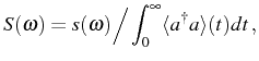
$\displaystyle S(\omega)=s(\omega)\Big/\int_0^\infty\langle\ud{a}a\rangle(t)dt\,,$

(2.75)

so that Eq. (2.75) is now the density of probability that a photon emitted by the system has frequency $\omega$ . This is independent of the detection time, in the same way as $\langle\ud{a}a\rangle (t)$ in Eq. (2.5) was the probability of emission of a photons disregarding their frequency. The Fourier transform of $a(\omega)=\int_0^{\infty}e^{i\omega t}a(t)dt/\sqrt{2\pi}$ relates the emission spectrum to a two-time correlator

$\displaystyle S(\omega)=\frac{1}{2\pi}\frac{1}{\int_0^\infty\langle\ud{a}a\rang... ...\iint_0^{\infty}\langle\ud{a}(t_1)a(t_2)\rangle e^{i\omega(t_2-t_1)}dt_1dt_2\,.$

(2.76)

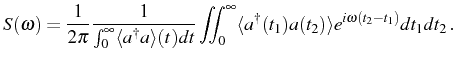
After a change of variables, $S(\omega)$ can be expressed in terms of the so-called first-order correlation function

$\displaystyle G^{(1)}(t,\tau)=\langle\ud{a}(t)a(t+\tau)\rangle$

(2.77)

at positive time delays $\tau=t_2-t_1>0$ . All put together, this yields the Fourier-pair relationship between the power spectrum and the correlation function, as used by Carmichael et al. (1989) and discussed in the introduction:

$\displaystyle S(\omega)=\frac{1}{\pi\int_{0}^\infty\langle\ud{a}a\rangle(t)dt}\Re\int_0^\infty\int_0^\infty G^{(1)}(t,\tau)e^{i\omega\tau}\,d\tau dt\,.$

(2.78)

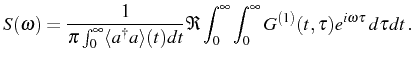
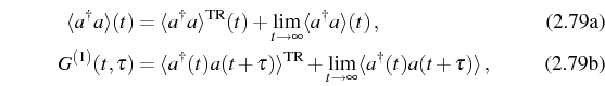
In the SS case, care must be taken with cancellation of infinities brought by the ever-increasing time

. Both the numerator and the denominator become infinite quantities. Their ratio, however, produces a finite quantity, which recovers the well-established and rigorously derived Wiener-Khintchine formula (see Mandel & Wolf (1995) discussion), that reads:^2.11

$\displaystyle S^\mathrm{SS}(\omega)=\frac{1}{\pi}\frac{1}{n_a^\mathrm{SS}}\Re\int_{0}^{\infty}G_\mathrm{SS}^{(1)}(\tau)e^{i\omega\tau}d\tau\,.$

(2.79)

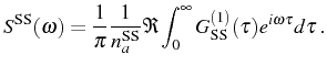
From the general Eq. (2.74) to the SS, Eq. (2.79), there is the cancellation of the diverging quantities by obtaining the final result as a limit of the time-integrated spectrum. The population and the correlator can be decomposed as a transient (TR) and steady-state (SS) values:

$\begin{subequations}\begin{align}\langle\ud{a}a\rangle(t)&=\langle\ud{a}a\rangle... ...ghtarrow\infty}\langle\ud{a}(t)a(t+\tau)\rangle\,, \end{align}\end{subequations}$

where $\lim_{t\rightarrow\infty}\langle\ud{a}a\rangle(t)=n_a^\mathrm{SS}$ . We rewrite Eq. (2.78) as the time integration of the Fourier transform until time

, that is left to increase without bounds:

$\displaystyle S(\omega)=\lim_{T\rightarrow\infty}\frac{1}{\pi\int_{0}^T\langle\... ...\Re\int_{t=0}^T\int_{\tau=0}^\infty G^{(1)}(t,\tau)e^{i\omega\tau}\,d\tau dt\,.$

(2.81)

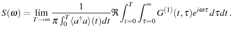
Substituting Eq. (2.80) in this expression, we can keep track of the terms that cancel (one can check a posteriori from the explicit results, the convergence of $N\equiv\int_0^\infty\langle\ud{a}a\rangle^\mathrm{TR}(t)dt$ and $M_\tau=\int_0^\infty\langle\ud{a}(t)a(t+\tau)\rangle^\mathrm{TR}e^{i\omega\tau}\,dt$ , for all $\tau>0$ ):

$\displaystyle S^\mathrm{SS}(\omega)=\frac{1}{\pi}\lim_{T\rightarrow\infty}\frac... ...\rightarrow\infty}\langle\ud{a}(t)a(t+\tau)\rangle\bigg]e^{i\omega\tau}d\tau\,.$

(2.82)

Since the norm of the Fourier transform of $M_\tau$ is also bounded (that, again, can be checked from the explicit result), the limit in

yields Eq. (2.79).

This discussion should motivate the physical meaning and validity of both formulas, and show the connections between them.

The first order cross correlation between two different field ( and ),

$\displaystyle G_{ab}^{(1)}(t,\tau)=\langle\ud{a}(t)b(t+\tau)\rangle$

(2.83)

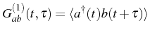
produces the spectral counterpart of Eq. (2.78), the so-called cross correlation function:

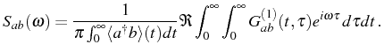
$\displaystyle S_{ab}(\omega)=\frac{1}{\pi\int_{0}^\infty\langle\ud{a}b\rangle(t)dt}\Re\int_0^\infty\int_0^\infty G_{ab}^{(1)}(t,\tau)e^{i\omega\tau}\,d\tau dt\,.$

(2.84)

This spectral function contains similar information than the power spectrum and can be also experimentally measured and analyzed, as has been argued by Karlovich & (2007).

Subsections