Cavity QED (cQED)

Cavity QED (cQED) rests on the realization above that the lifetime of an atom is not a property of the atom itself but of the coupled atom-radiation field system. If one would be able to alter the radiation field in some sense, such as for instance by suppressing its fluctuations (including those of the vacuum!) or modifying its density of states, this would alter the lifetime of an excited state, as suggested by Eq. (1.1) if $\rho(\omega)$ is changed.

The effect was first put to use by Purcell (1946) in nuclear magnetic resonance for the practical purpose of thermalizing spins at radio frequencies, by bringing down their relaxation time from $\approx10^{21}$ s to a few minutes. Interestingly, this seminal achievement in tailoring what was widely regarded before (since Einstein's theory of spontaneous emission) as an intrinsic property of matter, did not impress much Purcell himself or his contemporaries, despite the good timing (Purcell did not attend the Shelter Island conference, but Rabi, his then hierarchic superior, did). The effect of tailoring lifetime through the density of optical modes is nevertheless now known as the Purcell effect. Similar concepts were investigated from a more fundamental angle by Casimir (1948), for instance demonstrating the attraction between two conducting plates close enough for--in the words of Casimir--``the zero point pressure of electromagnetic waves'' being reduced between the plates. With regard to SE, the problem was considered again for its own sake by Kleppner (1981). In his initial proposal, he considered it in the opposite sense than Purcell, namely, to increase the lifetime of the excited state, by decoupling it from the optical field (and therefore also from its vacuum fluctuations). Soon after, Goy et al. (1983), from the Haroche group, reported the first experimental observation of Purcell enhancement.^1.8 The authors concluded their paper setting the goal for a higher milestone of cavity QED: when spontaneous emission is enhanced so much that absorption--which is equal to it from Einstein's theory--or more specifically, since we have only one emitter, reabsorption of the photon by its own emitter, becomes dominant over the leakage of the photon out of the cavity, then the perturbative--so-called Weak Coupling (WC)--regime breaks down and instead Strong Coupling (SC) takes place. In this case, emitted photons engage a whole sequence of absorptions and emissions, known as Rabi oscillations, until their ultimate decay out of the cavity. This regime is of greater interest, as it gives rise to new quantum states of the light-matter coupled system, sometimes referred to as dressed states (especially in atomic physics) or as polaritons (especially in solid-state physics). Experimentally, SC is more difficult to reach, as it requires a fine control of the quantum coupling between the bare modes and in particular to reduce as much as possible all the sources of dissipation.

Haroche's group in their first report of tuning the SE, placed this higher goal only ``a tenfold increase in '' away. Shortly after, they reported, with Kaluzny et al. (1983), the first observations of Rabi oscillations. However, rather than increasing the , they had used atoms, thereby enhancing the coupling strength by a factor $\sqrt{N}$ . Unfortunately, my thesis does not explore in its full generality the so-called Dicke Hamiltonian, that explains this enhancement. However we shall see its manifestation in the particular case of in Chapter 6. Haroche & Kleppner (1989) wrote an authoritative review on the early cQED experimental achievements.^1.9

On the theoretical side, Sanchez-Mondragon et al. (1983) were the first to address the fundamental problem of the lineshape of the SE in cQED.^1.10 They met with the difficulty of the definition of the optical spectrum, which had otherwise found an acceptable solution for physicists with the mathematical work of Wiener (1930) and Khinchin, even in the cases of non-stationary signals. But instead, under the guidance of Eberly, they had recourse to the more rigorous Eberly & Wodkiewicz (1977) time-dependent physical spectrum:

$\displaystyle \mathcal{R}(t,\omega_f)=\Gamma_f^2\int_{-\infty}^t\int_{-\infty}^... ..._1)}e^{-(\Gamma_f+i\omega_f)(t-t_2)}\langle\ud{a(t_1)}a(t_2)\rangle dt_1dt_2\,.$

(1.3)

This expression is derived from physical (rather than mathematical) grounds, computing probabilities of measuring a photon by absorption from a detector, that introduces its linewidth $\Gamma_f$ into the problem. The rest of their treatment was otherwise very straightforward. Their Hamiltonian was JC's and they considered as initial conditions the excited state of an atom in an empty cavity (case of Fig. 1.1) or in a cavity prepared in a coherent state, in which case they observed the transition from a Rabi doublet to a Mollow triplet with the intensity of light. This first description however suffered from serious limitations, the most important of which being the absence of dissipation: they considered an infinite lifetime atom in a lossless cavity (whence the ``ideal'' cavity). This is another value of Eberly and Wódkiewicz's approach that it takes into account the linewidth of the detector, thereby rescuing their result in such approximations, with well-behaved spectral-shapes rather than $\delta$ singularities. The doublet they obtained as a result of this modelization consists of exactly two Lorentzian lines. They could observe, however, the vacuum Rabi splitting and the anticrossing at resonance, but their result actually relates to the Hamiltonian structure of the coupling, artificially broadened. Their description is lacking in particular the most important feature of SE, as should be clear from our previous discussion, namely, irreversibility.

**Figure 1.1:** The first theoretical computation of the cQED lineshape of the spontaneous emission of a system in strong coupling, as detuned is varied, by Sanchez-Mondragon et al. (1983).
$\includegraphics[width=.5\linewidth]{introduction/sanchezmondragon-2.ps}$

If only for reasons of self-consistency, cavity decay should be included to describe any luminescence experiment, since photons should leak out from the cavity to be detected, as duly noted by Agarwal & Puri (1986), who added this ingredient $\gamma_a$ ( $\kappa$ in their notations) in a master equation for the coupled light-matter system:

$\displaystyle \partial_t\rho=-i[H,\rho]+\frac{\gamma_a}{2}(2a\rho\ud{a}-\ud{a}a\rho-\rho\ud{a}a)\,.$

(1.4)

is still JC Hamiltonian [Eq. (1.2)] although here, it is solved in the linear case, that is, considering only a maximum of one photon in the cavity. This constriction makes the problem equivalent to the linear model where both fields obey Bose algebra: two harmonic oscillators instead of a two-level atom (as we will see in Chapter 3). Moreover, in this limit of SE, the Lindblad form is not needed to compute correlator functions and a much more straightforward treatment is obtained by including dissipation as an imaginary part to the energy, as we shall also prove later. Interestingly, they used the same Eberly and Wódkiewicz' physical spectrum, Eq. (1.3). Agarwal & Puri (1986) also considered transmission and absorption as well as SE, but I will not discuss this aspect of their work, which is not directly related to the topic of this thesis, the photoluminescence (PL). Their PL results can be seen in Fig. 1.2.

**Figure 1.2:** Lineshapes of a coupled light-matter system with cavity dissipation, as computed by Agarwal & Puri (1986). Solid lines are cavity emission and dashed lines direct atomic emission. Detector linewidth was taken as (a) at resonance for no cavity decay (upper lines) and small cavity decay (lower lines). The strong coupling results in the Rabi doublet. (b) Same as (a) but for a detuning of . (c) Bad-cavity case with disappearance of the doublet.
$\includegraphics[width=\linewidth]{introduction/agarwal.ps}$

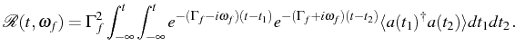
The most complete quantum optical calculation, supported by the most insightful discussion, was brought by Carmichael et al. (1989), who considered the most general case with both types of decay:

$\displaystyle \partial_t\rho=-i[H,\rho] +\frac{\gamma_a}{2}(2a\rho\ud{a}-\ud{a}a\rho-\rho\ud{a}a)$
$\displaystyle +\frac{\gamma_\sigma}{2}(2\sigma\rho\ud{\sigma}-\ud{\sigma}\sigma\rho-\rho\ud{\sigma}\sigma)\,.$	(1.5)

( $\kappa$ for the atom and $\gamma$ for the decay in their notations.) As their predecessors, the authors considered the SE of the initial state $\ket{e,0}$ (excited state, no photon in the cavity) and solved the problem exactly, thanks to the mapping with the linear model. In this case, the Hilbert space truncates to $\ket{e,0}$ , $\ket{g,1}$ , $\ket{g,0}$ . Their results can be seen in Fig. 1.3.

**Figure 1.3:** Lineshapes of a coupled light-matter system with both cavity and emitter dissipation, as computed by Carmichael et al. (1989), showing the subnatural linewidht averaging. Parameters are $\gamma_a\gg\gamma_\sigma$ and $2g/\gamma_\sigma=5$ . In inset, zoom on one peak comparing the SE (dashed), free-space fluorescence (broader line, dot-dashed) and fluorescence (solid).
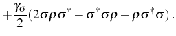
$\includegraphics[width=.5\linewidth]{introduction/carmichael.ps}$

In contrat with the two previous approaches, the PL spectrum was here computed with the formula:

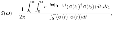
$\displaystyle S(\omega)=\frac{1}{2\pi} \frac{\displaystyle\int_0^\infty\int_0^\... ...2)\rangle dt_1dt_2} {\int_0^\infty \langle\ud{\sigma(t)}\sigma(t)\rangle dt}\,,$

(1.6)

which is the expression we shall later adopt in the case of time-dependent dynamics (case of SE) for several reasons. The main one is that the description of luminescence of the coupled light-matter system by Carmichael et al. (1989) is the most involved at this level of description and the one that, with Laussy et al. (2008b), I took as a starting point to formulate the counterpart of this problem for semiconductors. Another reason is that it frees us from the detector's linewidth, which does not need to enter the picture at a primary level, as it did in the two previous descriptions. It could be included in any case by the usual procedure of convolution. Finally, I will show later that formula (1.6) leads to the relevant case of the Wiener-Khinchin formula for the stationary fields.

Before closing this Section of the seminal experimental and theoretical efforts in cQED that are the most relevant for our subsequent discussion, I want to comment on the features that are missing from Carmichael et al. (1989)'s description for my purposes, and that I will provide in Chapter 3. Those are the arbitrary initial condition (rather than merely the excited state of the atom), and observation of the cavity emission (rather than only the direct atom emission). The later case means computing Eq. (1.6) with operators rather than $\sigma$ , and should be an obvious requisite to the semiconductor microcavity physicist. In their partial pictures, both Sanchez-Mondragon et al. (1983) and Agarwal & Puri (1986) had addressed these questions to some extent (but still far from full generality). The former had considered various coherent states of the optical field, and the latter had computed both the photon and exciton emission. I want to comment quickly on the necessity of these extensions, though we shall discuss them at greater length when I will address the problem head on. It is clear that the initial condition strongly influences the optical spectrum, as can be seen by considering as initial states the excited state of the atom, $\ket{e,0}$ , or one photon, $\ket{g,1}$ on the one hand, and an eigenstate of the Hamiltonian in Eq. (1.2), $\ket{e,0}\pm\ket{g,1}$ , on the other hand. These will normally (in SC) produce, a two Rabi peaks and only one of them, respectively, which are quantitatively very different. It is maybe less obvious that $\ket{e,0}$ and $\ket{g,1}$ , also differ in their SE when $\gamma_a\neq\gamma_\sigma$ , and in some case also quantitatively. These considerations, that in this context might appear as mere generalizations, will become a natural, and in fact, compulsory, requirement in the semiconductor treatment, to which I now turn.