Contents |
Computación I: Data Analysis
Data and its analysis
We live in the information age. Data is everywhere. Since our scientific method got based on experiment, starting with Galileo, we came to measure increasing numbers of variables in an increasing amount. The CERN generates over petabytes of data in single experiments and now records about several GigaBytes every second. Not only fundamental physics is subject to producing data but everything around us. Our every move get increasingly recorded and stored, even Adélie penguins are now weighted each time they are on their way to or from the sea. There is the need to bring meaning to such massive amounts of raw information, a field known as data mining. Unknown and often even unsuspected patterns exist in the world around us that fundamental models are too crude to describe, but that simple descriptive analysis can reveal. For instance, the darkening of books of logarithms for pages with smaller leading integers led to the realization of Benford's law, that in "natural data", the distribution of the leading digit is decreasing for smaller numbers, i.e., numbers starting with 1 are more frequent than those starting with 2, in turn more frequent than those starting with 3, etc., till 9, the least represented number. This is a shocking fact of our surrounding environment as our intuition strongly suggests on several acconts that they should be uniform! As a species, we want to learn the why and how of such things, and put them to practical use. In the case of Benford's law, for instance, this is used for fiscal fraud detection.

The mean
Bringing meaning means reducing the whole lot to a few quintessential quantities. A large set of points $x_i$, $1\le i\le N$, can indeed be reduced to such a few quantities that represent it roughly and, when successful, well enough. With no prior knowledge of the points, it is basically impossible to decide which are the good quantities. Remarkably, in many cases, a couple of quantities is enough to basically describe exactly the entire set!
The most basic such quantity is the central tendency, that aims at representing the typical value for a set. In absence of previous knowledge, this is almost invariably computed as an average, the simplest version of which is the arithmetic mean:
$$\bar x=\frac{1}{N}\sum_{i=1}^N x_i\,.$$
For instance, what is the sum of the first 100 integers? (question once put in an 18th century elementary school and solved mentally by a young Gauss.)
>> sum(1:100)

ans =

        5050
Gauss certainly pictured something like this:
plot((1:100),'bo')
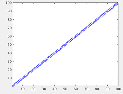
The story goes that he realized each number is paired with its symmetric about the center point, 0+100, 1+99, 2+98, etc., till 48+52 and 50 in isolation. They all sum up to 100 so we have 50 pairs of 100 + 50 itself, making 5050.
Possibly, Gauss saw it this way: this sum is 100 times the average, which is the center of the $y$ axis on this plot, that goes from 1 to 100, i.e., 101/2. From this argument one easily get the general formula\[\overline{[1,N]}=\frac{N(N+1)}{2}\,.\]
The mean in matlab is, by the way, mean():
>> 100*mean(1:100)

ans =

        5050
What is the mean value of a set of random points? Of course this depends from their distribution. If they are random beween 0 and 1, that should be 0.5.
>> rand10=rand(10,1)'

rand10 =

    0.6876    0.2164    0.3474    0.7492    0.2914    0.0123    0.0009    0.0123    0.0682    0.6173

>> mean(rand10)

ans =

    0.3003
Not quite close... This is due to a fluctuation.
Fluctuations
The fact our random number fluctuate (of course) will give us a natural nontrivial source of data. We will in the following study such data. You are now and henceforth encouraged to play statistics with all the data you will encounter on a daily basis.
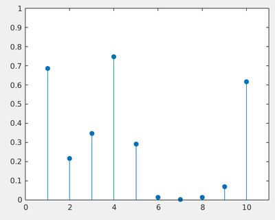
By "poor luck", we had, above, an anomalous large number of small numbers. Such effects would disappear with "better statistics", which means here, more points. The same with 100 points:
>> stem(rand(100,1),'filled')
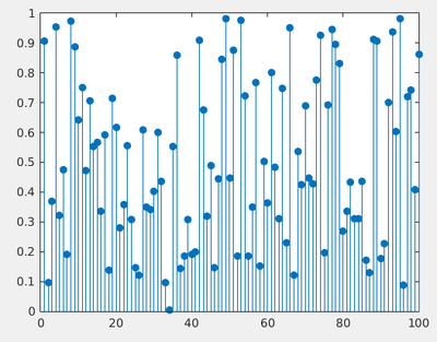
The average for the above is 0.5074.
How close we are from the expected mean is the second quantity that describes our set of points, and that quantifies its dispersion.
Let us write a matlab program to explore numerically how do the average fluctuate around its expected mean as a function of the size of the sample.
For one given sample size, to get some idea:
n = 100; % Number of averages
devmean = zeros(1, n);  % pre-allocation
for k = 1:n
  devmean(k) = mean(rand(10,1));    % Average over 10 numbers
end
plot(devmean)
axis([-inf inf 0 1])
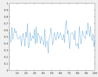
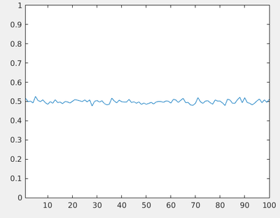
This is the same but now averaging over 100 numbers:
The Normal distribution
We see there are less fluctuations. How to measure that? Let us first get a sense of how these particles are distributed, by plotting, precisely, their distribution:
n = 1000; % Number of averages
devmean = zeros(1, n);  % pre-allocation
for k = 1:n
  devmean(k) = mean(rand(10,1));    % Average over 10 numbers
end

partition = [0:.05:1]; % Binning
distribution = histcounts(devmean,partition,'Normalization', 'probability');
bar(linspace(0,1,length(distribution)),distribution)
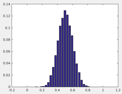
This distribution should be familiar. If not, it has to become so, because it is one of the most important object of our physical universe. This is the Normal distribution, also known as a Gaussian. This is the distribution that reduces essentially exactly a large set of points to two numbers:
- The mean.
- The standard deviation.
Note that such concepts are valid for Normal distribution of points, which do not cover all (but most) cases. For instance, averaging over 2 numbers does not lead to a Normal distribution of the averages:
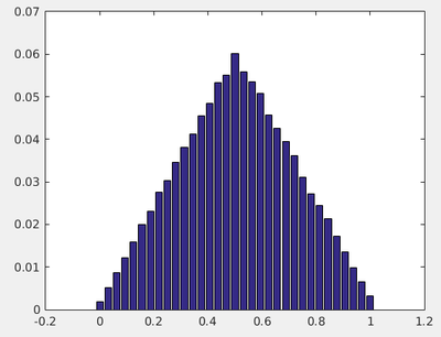
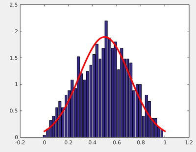
In probability theory, one can show that the sum of two independent random variables follows the distribution given by the convolution of the distribution of the random variables, which explains this triangular shape.
Maybe you can guess on logical grounds what would be the distribution when getting down to one number?
Back to our initial problem of quantifying the dispersion of the average depending on the sample's size: clearly, we can use the standard deviation of the Normal distribution. How to obtain it from the distribution itself, though? We could fit the function. This is the approach we will take in next lecture when we learn data fitting. For now, we will use what is known in statistics as an estimator, i.e., a formula that provides the standard deviation from the points directly. One can show that for points normally distributed\[s=\sqrt{\frac{1}{N-1}\sum_{i=1}^N(x_i-\bar x)^2}\,.\]
Here you must pay attention that the formula differs slightly from the standard deviation defined as the square root of the variance\[\sigma=\sqrt{\frac{1}{N}\sum_{i=1}^N(x_i-\bar x)^2}\,.\]
This does not matter when the size of the sample is large enough. In our case over 10 averages:
>> sqrt(sum((devmean-mean(devmean)).^2)/length(devmean))

ans =

    0.0899
which is the same as dividing by $N-1$. In matlab, the standard deviation can be calculated by std():
>> std([1 2 3 4 5])

ans =

    1.5811

>> std([1 2 3 4 5],1)

ans =

    1.4142
The second example uses the variance. The sample is small, so there is a difference in this case. The two definitions come from the theory of statistical inference, that aims at describing large sets through smaller samples. It so happens (as can be demonstrated, but this is outside the scope of this lecture) that dividing by $N$ leads to an underestimation of the real spread (the correction of $-1$ comes from Bessel). We will come back to this point (see also the projects). In the meantime, We continue to explore this idea with our initial goal of getting the dispersion of the mean as function of the size of the sample. For this, it may be convenient to define a function. In a file devmean.m we write the function:
% return the standard deviation of numAverage averages over samples of size sampleSize

function res = devmean(sampleSize,numAverage)

devmean = zeros(1, numAverage);  % pre-allocation
for k = 1:numAverage
  devmean(k) = mean(rand(sampleSize,1));    % Average over sample size
end
res = std(devmean);
end
that we call in a different script:
pop = [1 10 100 1000 10000 100000];
myeststd = zeros(length(pop),1);
for i = 1:length(pop)
    fprintf('Processing size %d ...', pop(i));
    myeststd(i)=standdev(pop(i),1000);
    fprintf(' Done.\n');
end
loglog(pop,myeststd,'-o');
xlabel('Size of sample');
ylabel('Standard deviation of mean');
$\tag{1}\nonumber$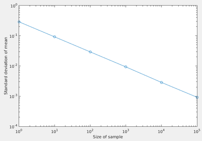
Figure (1)
This is a result, so we spare a minute to label the axes and make it a figure of its own, independent of the flow of the text. In next lecture, we will identify what the exact relation is.
Until then, we can check the consistency of our previous statements by comparing theory with (our numerical) experiments. We first need to remind the analytical expressions for the Gaussian\[ f(x)=\frac{1}{\sqrt{2\pi\sigma_x^2}}\exp\left(-\frac{(x-x_0)^2}{2\sigma_x^2}\right)\,, \]
We now plot together this formula with the standard deviation calculated from the points, along with a distribution of the points obtained by binning:
lnSample=1000;
randSamp = zeros(lnSample,1);
sampSize = 10;

for i=1:lnSample
randSamp(i)=mean(rand(sampSize,1));
end

minx=0;
maxx=1;
dx=0.025;

partition = [minx:dx:maxx];
distribution = histcounts(randSamp,partition,'Normalization', 'probability');

clf;
bar(linspace(minx,maxx,length(distribution)),distribution/dx)
hold on;

sx=devmean(sampSize,1000);
x=linspace(0,1,100);
y=(1/(sqrt(2*pi*sx^2)))*exp(-(x-0.5).^2/(2*sx^2));
plot(x,y,'LineWidth',3,'Color','red')
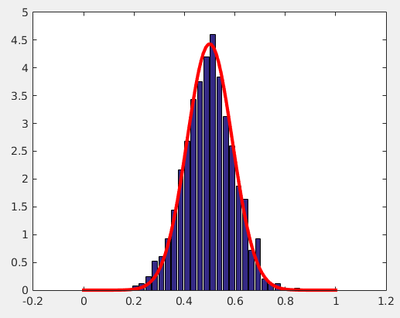
It works quite well. In fact, it works surprisingly well. Even for averages over two numbers, for which we know this is not normally distributed, we get a fair agreement:
Normal and Standard
The normal distribution is by far the most common one (hence the name, normal). We have seen at least two others already:
- The uniform distribution (with which we have generated the data giving rise to the normal distribution).
- The triangular distribution (when taking a particular case of averaging over two numbers).
These distributions can be generated directly by matlab (we already know rand() that generate uniform numbers):
>> plot(normrnd(.5,.1,100,1))
axis([-inf inf 0 1])
It is important, to make sense of statistics, to understand well the Normal distribution and its properties. For instance, the standard deviation is popularly given some visibility through error bars. This is a fairly subtle concept that is sometimes mistreated by its careless application.
Let us compare, for instance, the "$N$ and $N-1$ definitions" of the standard deviation for small samples (up to 25 points), by showing the statistical spread in this way:
totpts=10;

lav=zeros(1,totpts);
lstdN=zeros(1,totpts);
lstdNm1=zeros(1,totpts);

for numpts=1:totpts
    pts=normrnd(0,.1,numpts,1);
    lav(numpts)=mean(pts);
    lstdN(numpts)=std(pts,1);
    lstdNm1(numpts)=std(pts);
end

hold off
errorbar(lav,lstdN)
axis([0 totpts -1 1]);
hold on
errorbar(lav,lstdNm1)
xlabel('Size of sample');
ylabel('Mean (+error)');
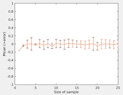
Here we have a real numerical experiment, and it was easy enough to put error bars (using errorbar(), calculated by matlab itself). This makes a nice graphics. What is its meaning, however? The ideal result is an average of 0 with a deviation of 0.1 (as we have written in the code). This is realized for points on the right. Points on the left would appear to the naive high to be better points. The error is generally smaller. It is zero for the first point. This, however, only reflects the few statistics available, leading to possible small variance. Note also the little importance, in this case, of the Bessel correction.
An "abnormal" distribution
We will now study another fundamental distribution, that behaves very differently. In matlab, it comes by the name trnd(1):
>> trnd(1)

ans =

    0.3269
This shows a statistics of 100 realizations:
stem(trnd(1,100,1),'filled')
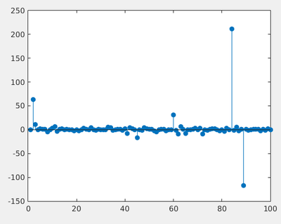
This distribution is known as the Cauchy distribution (its name in matlab is due to it being a particular case, when $\nu=1$, of the $t$-Student distribution). It is very different to the behaviour or the normal distribution, in that it fluctuates to all orders. This means that once in a while, a point will lie very far from the cloud of the others. Such points are known as outliers. On the contrary, "normal" fluctuations are contained within their interval of standard deviation. Outliers there, although still possible, are so improbable that they are considered errors.
The functional form of the Cauchy distribution is a Lorentzian. It is a basic lineshape of fundamental physics (the Fourier transform of the exponential, which corresponds to memoryless decay). It is also a paradigmatic object of the black swan theory.
randCauchy=trnd(1,100000000,1);

partition = [-10000:10:10000]; % Binning
distribution = histcounts(randCauchy,partition,'Normalization', 'probability');
bar(linspace(-10000,10000,length(distribution)),distribution)
set(gca,'YScale','log')
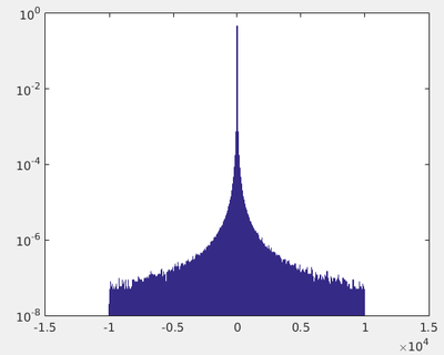
Its main feature is the "fat tails" that shows how, for enough repetition of our luck, we eventually fluctuate far enough. The above distribution is the same over 100 million points as the previous figure that considered 100 points only, with maximum absolute fluctuation less than 150. We have truncated the binning. The larger set in fact went as far as:
>> min(randCauchy)

ans =

  -9.4912e+08

>> max(randCauchy)

ans =

   6.6095e+07
That is, ten thousand time farther than what is shown on the plot.
This is an example of a distribution that cannot be characterized by a standard deviation. It cannot even be characterized by its mean, it does not have any! By sampling from this distribution, eventually, an outlier will by itself overrule all the other points of the set, thus spoiling the concept of average. The mean itself will not be normally distributed!
Other statistical indicators
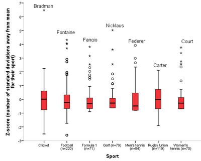
This failure of the mean is common in complex systems. For instance, in a human's society, it is typically useless (or deceptive) to consider the mean when speaking of, e.g., wealth. A rich man is somebody's else poor. The average person's wealth in a city is typically that of the richest person. The following graph shows how a similar concept now in sport, with the most important departure ever noted being in cricket (from [1]):
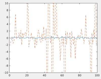
Still we have to characterize our set of points in a useful way. A popular replacement to the mean is the median, defined as the value for which half the points have a smaller value and the other half have a larger value.
med=zeros(1,100);
for i=1:100
    med(i)=median(trnd(1,100,1));
end
plot(med)
axis([0 100 -1 1])
Another popular replacement for the mean is the mode, defined as the most common value of the set (the maximum point in a distribution probability), but this is for statisticians rather than physicists and mathematicians.
The study of the statistical properties of such quantities derived from samples of a larger population ruled by an hypothetical rule is the topic of an entire field of its own: inferential statistics. One proposed project will delve into more details of this and related problems. In the meantime, we can carry on our explorations and analysis. We have considered above the simple case of the distribution of the mean of random numbers. What is the distribution of the mean of the square of $k$ numbers? Do you have an a-priori intuition?
Let us explore:
numsum=1;
numpts=10000;
sumsq=zeros(numpts,1);

for i=1:numpts
    sumsq(i)=mean(rand(numsum,1).^2);
end

partition = [0:.01:1]; % Binning
distribution = histcounts(sumsq,partition,'Normalization', 'probability');
bar(linspace(0,1,length(distribution)),distribution)
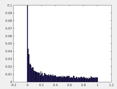
We see that qualitatively different results are obtained for different sample-size. In particular, if we consider not uniformly distributed but normally distributed numbers, we reach a fundamental and already quite advanced object of statistical theory. We will learn about it in next lecture.
| Computación I |
|---|
|