

Two quantum dots in a microcavity
![\includegraphics[width=0.8\linewidth]{chap6/2P/Levels/levels-no-biexc.eps}](img1716.png)
We consider that the two QDs of Chapter 4 are not
directly coupled but each of them interacts separately with the same
cavity mode, with coupling strengths ![]() and
and ![]() . In general, the
modes are not at resonance but detuned by a small quantity
. In general, the
modes are not at resonance but detuned by a small quantity
![]() ,
, ![]() , 2, from the cavity
mode
, 2, from the cavity
mode ![]() . These four parameters
. These four parameters
![]() and
and
![]() represent the experimental inhomogeneity
present in the sample. The total Hamiltonian in this case is the sum
of two Jaynes-Cummings Hamiltonians, a particular case of the
so-called Dicke Hamiltonian for only two emitters:
represent the experimental inhomogeneity
present in the sample. The total Hamiltonian in this case is the sum
of two Jaynes-Cummings Hamiltonians, a particular case of the
so-called Dicke Hamiltonian for only two emitters:
![$\displaystyle H= \omega_a \ud{a}a + \sum_{i=1,2} [\omega_i \ud{\sigma_i}\sigma_i + g_i \big( a\ud{\sigma_i} + \ud{a} \sigma_i \big) ] .$](img1723.png)
The QD levels as compared with the cavity mode are plotted in Fig. 6.1. Together with this ``localized'' QD basis of states, that we already introduced in Chapter 4, one can refer to the Dicke states, corresponding to the triplet states:
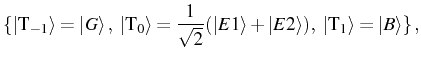
and to the singlet state
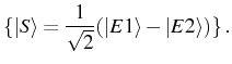
In the Dicke basis, the interaction part of
where
![\includegraphics[width=\linewidth]{chap6/fig_1.eps}](img1734.png) |
The master equation of the system includes decay for both the cavity
mode and the QDs. The QD leaky parameters are set to
![]() , a value much smaller than the
typical cavity decay rates
, a value much smaller than the
typical cavity decay rates ![]() considered and experimentally
achievable in general. We neglect pure dephasing of the QDs for
simplicity. The pumping scheme is the most important ingredient in
this work. We consider two physically different situations that we
explain in what follows, deriving the appropriate Lindblad terms from
the microscopic approach.
considered and experimentally
achievable in general. We neglect pure dephasing of the QDs for
simplicity. The pumping scheme is the most important ingredient in
this work. We consider two physically different situations that we
explain in what follows, deriving the appropriate Lindblad terms from
the microscopic approach.
First, the case where the two QDs are distinguishable in a classical
(as opposed to ``quantum'') way for the pump excitation. Such a
situation arises when both QDs are far enough from each other to be
resolved and pumped independently or have very different excitation
energies. This is the case when the collection areas around
each dot--the areas of the wetting layer where free carriers are
captured by the dot--are completely separated. In the following we
denote by ![]() the collection areas of the dots (considered equal for
simplicity) and
the collection areas of the dots (considered equal for
simplicity) and ![]() their overlapping area. Each of the QDs couple
independently to each element of its own reservoir
(electrons
their overlapping area. Each of the QDs couple
independently to each element of its own reservoir
(electrons ![]() , holes
, holes ![]() and phonons
and phonons ![]() ), with
coupling strengths
), with
coupling strengths
![]() . This is the situation encountered
with atoms and that has been more systematically explored. The
Hamiltonian of such a coupling reads:
. This is the situation encountered
with atoms and that has been more systematically explored. The
Hamiltonian of such a coupling reads:
![$\displaystyle H_\mathrm{pump} = \sum_{R_1} \big[ \, \delta_{R_1} \ud{\sigma_1} ...
...elta_{R_2} \ud{\sigma_2}\, e_{R_2} h_{R_2}\ud{f_{R_2}} + \mathrm{h.c.} \big]\,.$](img1741.png)
Applying the method and approximations described in Chapter 2, Sec. 2.4, one arrives to two independent Lindblad terms of the form:
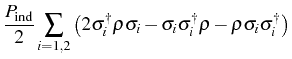
with parameters that we expect to be proportional to the collection areas
![\includegraphics[width=0.4\linewidth]{chap6/fig_2.eps}](img1745.png) |
On the other hand, when, e.g., two identical dots are close to each
other, if the coherence length of the excitation is larger than the
distance between the two dots, the final state is a quantum
superposition of the excited states of the QDs. This second situation
of a common excitation bath has been considered by
Braun (2002), keeping the coherent nature of the couplings
to the bath. An analogous scheme of a common reservoir has been
developed by Ficek & (2002) and by Akram et al. (2000), but
for a common squeezed vacuum. It requires the QDs to be
indistinguishable for the pumping mechanisms (with equal excitation
energies
![]() ), the reservoir
excitations--electron-hole pairs with high energy and phonons--to
have a large enough coherence length to be shared by both dots, and
the two collection areas to be fully overlapped (
), the reservoir
excitations--electron-hole pairs with high energy and phonons--to
have a large enough coherence length to be shared by both dots, and
the two collection areas to be fully overlapped (![]() ). With these
characteristics, there is only one common reservoir and, given that we
consider equal efficiencies for the dots (the excitation always
affects both dots in the same way), only symmetrical states can be
pumped. The Hamiltonian now reads:
). With these
characteristics, there is only one common reservoir and, given that we
consider equal efficiencies for the dots (the excitation always
affects both dots in the same way), only symmetrical states can be
pumped. The Hamiltonian now reads:
![$\displaystyle H_\mathrm{pump} = \sum_{R} \big[ \,\delta_{R}\big( \, \ud{\sigma_1} + \ud{\sigma_2}\,\big) e_{R} h_{R} \ud{f_{R}} + \mathrm{H.c.}\big]\,.$](img1748.png)
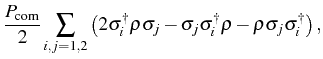
Taking into account the fact that the reservoir is common, we obtain two different contributions to the master equation:
- The first is an incoherent contribution to the dynamics given by
a Lindblad term:
with rate .
.
- The second is a direct coupling between the QDs which appears as
a coherent coupling in the Hamiltonian,
![$ H_{12}=g_{12} \big[ \,
\ud{\sigma_1} \sigma_2^- + \mathrm{H.c.} \, \big]$](img1751.png) with
with  of the order of magnitude of the common pumping
 . In the Dicke basis this coupling detunes the state
 from
from
 .
.
In a more general and realistic case, the collection areas overlap
partially in the region ![]() , which contributes to the common pumping
with a rate
, which contributes to the common pumping
with a rate
![]() , while the rest of the areas
, while the rest of the areas
![]() contribute to the excitation of each of the QDs separately
with rates
contribute to the excitation of each of the QDs separately
with rates
![]() (see
Fig. 6.3). We define the degree of common
pumping as the fraction
(see
Fig. 6.3). We define the degree of common
pumping as the fraction ![]() . Varying it between 0 and 1
interpolates between the two extreme cases of independent and common
pumping. The Lindblad term of the total pumping is separated in two
parts, one specific to each dot which depends on
. Varying it between 0 and 1
interpolates between the two extreme cases of independent and common
pumping. The Lindblad term of the total pumping is separated in two
parts, one specific to each dot which depends on
![]() and
another one which is invariant under QDs exchange (creates symmetrical
states) and that can be expressed in terms of the operator
and
another one which is invariant under QDs exchange (creates symmetrical
states) and that can be expressed in terms of the operator
![]() . The total master equation of the
system is now complete:
. The total master equation of the
system is now complete:
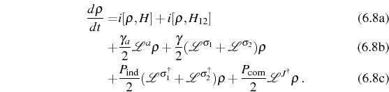
As a summary, the first line (6.9a) describes the coherent dynamics of the two dots and the cavity including the direct QD coupling created by the common excitation bath (
Here, we are interested in the properties of the steady state of
Eq. (6.9) in the limit of strong coupling between
cavity and QDs. This state was obtained in two independent and
equivalent ways. First we solved the set of linear equations for the
density matrix elements resulting from setting the time derivative to
zero
![]() . Second, we time-integrated the master equation and
waited a time long enough to reach the steady state. The solution is
unique for a given set of parameters, regardless of the initial state,
and both methods agreed exactly except when a singularity arises (as
detailed in the next Section) which can only be reached asymptotically
with the time-integrated approach.
. Second, we time-integrated the master equation and
waited a time long enough to reach the steady state. The solution is
unique for a given set of parameters, regardless of the initial state,
and both methods agreed exactly except when a singularity arises (as
detailed in the next Section) which can only be reached asymptotically
with the time-integrated approach.
Subsections Elena del Valle ©2009-2010-2011-2012.