Discussion

Although the spectra in the semiconductor case that are probed at negligible electronic pumping ( $P_b\ll1$ ) with no cavity pumping at all (), are in principle described by the same expression as that of the SE case used in the atomic model, in practise, however, both of these conditions can be easily violated. The renormalization of $\gamma_b$ with brings significant corrections well in the regime where , $n_b\ll 1$ and one could think that the pump is negligible. For instance, for parameters of point (c) in Fig. 3.9 with , the rate that is needed to bring a $100\%$ correction to $\gamma_b$ yields, according to Eqs. (3.15a) and (3.15b), average populations much below unity, namely, $n_a^\mathrm{SS}\approx0.026$ and $n_b^\mathrm{SS}\approx0.121$ . By the time reaches unity, with still one fourth smaller, the correction on the effective decay rate has became 400%. Because of thermal fluctuations in the particle numbers, for these average values, the results are already irreconcilable with a SE emission case. They are, as we shall see in the next Chapter, also irreconcilable with a Fermion model. As this is which is proportional to the signal detected in the laboratory, the electronic pumping must be kept very small so that corrections to the effective linewidth can be safely neglected. As regimes with high occupation numbers are reached, the renormalized $\Gamma$ s become very different from the bare $\gamma$ s in this model.

Second, even in the vanishing electronic pumping limit, it must be held true that is zero. Even if only an electronic pumping is supplied externally by the experiment, the pumping rates of the model are the effective excitation rates of the cavity and exciton field inside the cavity, and it is clear that photons get injected in the cavity in structures that consists of numerous spectator dots surrounding the one in SC (cf. Fig. 2.2). Although most of these dots are in WC and out of resonance with the cavity, they affect the dynamics of the SC QD by pouring cavity photons in the system. In the steady state, following our previous discussion, this corresponds to changing the effective quantum state for the emission of the strongly coupled QD. As we shall see in more detail in what follows, this bears huge consequences on the appearance of the emitted doublet, especially on its visibility.

To fully appreciate the importance and deep consequences of these two provisions made by the SS case on its SE counterpart, we devote the rest of this Section to a vivid representation in the space of pumping and decay rates. Now that it has been made clear what is the relationship between the SE and the SS cases, we shall focus on the latter that is the adequate, general formalism to describe SC of QDs in microcavities.

In presence of a continuous, incoherent pumping, the criterion for SC--from the requirement of energy splitting and oscillations in the $\tau$ dynamics that we have discussed above--gets upgraded from its usual expression found in the literature:

$\displaystyle g>\vert\gamma_-\vert\,,$

(3.65)

to the more general condition:

$\displaystyle g>\vert\Gamma_-\vert\,.$

(3.66)

The quantitative and qualitative implications and their extent are shown in Fig. 3.9, where we have fixed the parameters $\gamma_b=0.1g$ and , and outlined the various regions of interest as and $\gamma_a$ are varied (central panel). This choice of representation allows us to investigate configurations that can be easily imprinted experimentally in the system: by tuning in cavities that have different quality factors (inversely proportional to $\gamma_a$ ).

The red lines enclosing the filled regions in the central plot, delimit a frontier above which the pump is so high that populations diverge (there is no steady state). This is given by the equivalent conditions that we derived in two different ways, Eqs. (3.23) and (3.36). At resonance, they simplify to

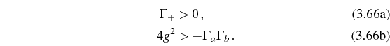
$\begin{subequations}\begin{align}\Gamma_+&>0\,,\\ 4g^2&>-\Gamma_a\Gamma_b\,. \end{align}\end{subequations}$

In the SC regime, the first condition is sufficient: $R_\mathrm{i}=0$ and the total decay rate for the system is given only by $\Gamma_+$ (condition (3.70b) is therefore automatically fulfilled). The equation for the border of the physical region in SC reads:

$\displaystyle P_b=\gamma_a+\gamma_b-P_a\,$ (boundary of SC) $\displaystyle .$

(3.68)

In the WC regime, condition (3.70b) becomes restrictive and the limiting value for

reads:

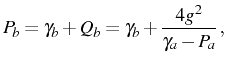$\displaystyle P_b=\gamma_b+Q_b=\gamma_b+\frac{4g^2}{\gamma_a-P_a}\,,$ (boundary of WC),

(3.69)

and can be interpreted as the point where the effective decay rate for mode

(direct losses plus its Purcell emission through mode

) is exactly counterbalanced by the effective pump [ $\Gamma_b^\mathrm{eff}=0$ , from Eq. (3.21)].

The main separation inside that region where a SS exists, is that between SC (in shades of blue, inside the triangle) and WC (in shades of red, on its right elbow). The blue solid line that marks this boundary, is specified by $g=\vert\Gamma_-\vert$ , i.e., by

$\displaystyle P_b=4g-\gamma_a+\gamma_b+P_a\,,$ (SS transition between SC and WC).

(3.70)

The dashed vertical black line, specified by $g=\vert\gamma_-\vert$ , i.e., by

$\displaystyle \gamma_a=4g+\gamma_b\,,$ (SE transition between SC and WC),

(3.71)

corresponds to the standard criterion of SC (without incoherent pumping).

The light-blue region, labelled 1 in Fig. 3.9, corresponds to SC as it is generally understood. The luminescence spectrum shows a clear splitting of the lines. The dark-blue region, labelled 2, corresponds to SC, according to the requisite that be real, but when in the luminescence spectrum, Eq. (3.63), only one peak is resolved. This region is delimited by the brown line, which is the solution of the equation $d^2S(\omega)/d\omega^2\vert _{\omega=0}=0$ , i.e., no concavity of the spectral line at the origin. From this condition follows the implicit equation:

$\displaystyle (3\Gamma_+-\Gamma_-)g^2+(\Gamma_--\Gamma_+)^3+g\vert D_0\vert(g^2-\Gamma_-^2+3\Gamma_+^2)=0$

(3.72)

that yields two solutions, only one of which is physical. The other one is placed on the red line $\Gamma_+=0$ , where the system diverges and the Rabi peaks become delta functions $\delta(\omega\pm g)$ . Note that this line extends into the WC region, as we shall discuss promptly. The distinction between the line-splitting in Eq. (3.66), as it results from the emergence of new dressed states in the SC, and the splitting observed in the spectrum given by Eq. (3.67), is seen clearly in Fig. 3.10. Here, the two are superimposed and seen to differ greatly even at a qualitative level for most of the range of parameters, coinciding only in a narrow region. The doublet, as observed in the luminescence spectrum, collapses much before SC is lost. Any estimation of system parameters, such as the coupling strength, from a naive interpretation of the peak separation in the PL spectrum, will most likely be off by a large amount.

**Figure 3.10:** Rabi splitting at resonance (dotted blue) given by $\pm \Re\{R_0\}$ , Eq. (3.33), and the observed position of the peaks in the PL spectra (solid red), Eq. (3.67), as a function of . Parameters are those of the line of points (a), (b) and (c) of Fig. 3.9: $\gamma_a=3.8g$ , $\gamma_b=0.1g$ , . The corresponding are marked for those points.
$\includegraphics[width=0.7\linewidth]{chap3/fig10-(a,b,c)-Splitting-with-Pb.eps}$

In Fig. 3.11, we plot, as a function of detuning the following magnitudes: in solid black, the bare modes ( $\omega_a=0$ , $\omega_b=-\Delta$ ); in dashed black, the dressed modes in the absence of pump and decay ( $\Re\{-\Delta/2\pm\mathcal{R}\}$ ); in dashed blue, the system dressed modes ( $\Re\{\Omega_\pm\}$ ); and in solid red, the actual splitting of the lines in the spectra given by the corresponding solutions of Eq. (3.52). We do this for the cases (a), (b), (c) and (e) of Fig. 3.9. By comparing with the blue polariton energy lines, it is clear that both the repulsion of the red lines in the spectra (cases c and e) and their crossing (cases a and b) can appear both in SC (b and c) or WC (a and e).

The last region of SC, labelled 3, is that specified by $4g+\gamma_b<\gamma_a<4g+\gamma_b+P_a-P_b$ , i.e., that which satisfies Eq. (3.69) but violates Eq. (3.68), thereby being in SC according to the more general definition that takes into account the effect of the incoherent pumping, but that, according to the conventional criterion, is in WC. For this reason, we refer to this region as of pump-aided strong coupling. This is a region of strong qualitative modification of the system, that should be in WC according to the intrinsic system parameters ( $\gamma_a,\gamma_b,g$ ), but that restores SC thanks to the cavity photons forced into the system.

**Figure 3.11:** Polariton splittings as a function of detuning for the cases (a), (b), (c), (e) of Fig. 3.9. Solid black: Bare energies of the cavity, $\omega_a=0$ , and exciton, $\omega_b=-\Delta$ , modes. Dashed black: Eigenenergies of the total system Hamiltonian, without dissipation nor pumping [ $-\Delta/2\pm \mathcal{R}$ , from Eq. (2.56a)]. Dotted blue: Positions of the underlying polariton modes, $\pm \Re\{\Omega_{\pm}\}$ , with the corresponding pump and decay. Solid red: Actual position of the observed peaks in the photoluminescence spectra given by the solutions of Eq. 3.52. Both repulsion (c and e) and crossing (a and b) of the (red) lines appear in SC (b and c) or WC (a and e), given by the splitting of the (blue) polariton energies.
$\includegraphics[width=.45\linewidth]{chap3/figa--Splitting-with-det.eps}$ $\includegraphics[width=.45\linewidth]{chap3/figb--Splitting-with-det.eps}$ $\includegraphics[width=.45\linewidth]{chap3/figc--Splitting-with-det.eps}$ $\includegraphics[width=.45\linewidth]{chap3/fige--Splitting-with-det.eps}$

We now consider the other side of the blue line, that displays the counterpart behavior in the WC. Region I is that of WC in its most natural expression. Region II, in light, is the extension into WC of featuring two maxima in the emission spectrum. In this case, this does not correspond to a line-splitting in the sense of SC where each peak is assigned to a renormalized (dressed) state, but rather to a resonance of the Fano type that is carving a hole in the single line of the weakly coupled system. In this region, one needs to be cautious not to read SC after the presence of two peaks at resonance. Finally, region III is the counterpart of region 3, in the sense that, according to the conventional criterion for the system parameters [Eq. (3.68)], this region is in SC when in reality the too-high electronic pumping has bleached it.

**Figure 3.12:** The same phase space of SC/WC as in Fig. 3.9 as a function of and $\gamma_a/g$ , only with now set to zero (no cavity pumping). The triangle of SC is displaced, and the regions of one peak spectra (regions 2 of SC and I of WC) are enlarged, following Eq. (3.75). As a result regions 3 and II have disappeared.
$\includegraphics[width=0.75\linewidth]{chap3/fig11-pyramid-2.eps}$

In the inset of Fig. 3.9's central panel, we reproduce the diagram to position the five points (a)-(e) in the various regions discussed, for which the luminescence spectra are displayed and decomposed into their Lorentzian (green lines) and dispersive (brown) contributions, Eqs. (3.55) and (3.57). Case (c), at the lower-left angle, corresponds to SC without any pathology nor surprise: the doublet in the luminescence spectrum--although displaced in position as shown in Fig. 3.10--is a faithful representation of the underlying Rabi-splitting. Increasing pumping brings the system into region 2 where, albeit still in SC, it does not feature a doublet anymore. The reason why, is clear on the corresponding decomposition of the spectrum, Fig. 3.9(b), with a broadening of the dressed states (in green) too large as compared to their splitting. Further increasing the pump brings it out of the SC region to reach point (a), where the two Lorentzians have collapsed on top of each other. This degeneracy of the mode emission means that the coupling only affects perturbatively each mode. As a result, the dispersive correction has vanished, and the spectrum now decomposes into two new Lorentzians centered at zero, with opposite signs [Eq. (3.64)].

Back to point (c), now keeping the pump constant and increasing $\gamma_a$ , we reach point (d). It is still in SC, although the cavity dissipation is very large (more than four times the coupling strength) for the small value of $\gamma_b$ considered. Its spectrum of emission shows, however, a clear line-splitting that is made neatly visible thanks to the cavity (residual) pumping . Note that the actual separations of the two peaks is much larger than that of the dressed states. Increasing further the dissipation eventually brings the system into WC, but in region II where, again due to $P_a\neq0$ , the spectrum remains a doublet. In Fig. (e), one can see, however, that there is no Rabi splitting, and that the two peaks arise as a result of a subtraction of the two Lorentzians centered at $\omega_a=0$ [see the WC spectrum decomposition in Eq. (3.57) and (3.64)]. Varying detuning for the system of point (e), even leads to an apparent anticrossing. There is no need to display a spectrum from region I, as in this case it does not show any qualitative difference as compared to that of (a). Note that the transition from SC to WC is always smooth in the observed spectra, although it is an abrupt transition in terms of apparition or disappearance of dressed states (due to a change of sign in a radical in the underlying mathematical formalism).

The schema in Fig. 3.9, constructed through Eqs. (3.71)-(3.75), contains all the physics of the system. In the following, we shall look at variations of this representation to clarify or illustrate those aspects that have been amply discussed before.

**Figure 3.13:** Phase space of SC/WC as a function of the pumps and for fixed decay parameters $\gamma_a=3.8g$ and $\gamma_b=0.1g$ . As in Fig. 3.9, the red lines mark the physical regions and the blue one the SC (blue shades)/WC (red shades) transition, with the same regions 1 and 2 of SC and III of WC, also with the points (a), (b) and (c), of Fig. 3.9. In inset, zoom of the low-pump region, showing the importance of both the angle, $\arctan{(1/\alpha)}$ , and the magnitude, $\sqrt{P_a^2+P_b^2}$ , of a given point in the diagram.
$\includegraphics[width=0.75\linewidth]{chap3/fig12-pyramid-3.eps}$

Fig. 3.12 shows the same diagram as that of Fig. 3.9, only with now set to zero, i.e., corresponding to the case of a very clean sample with no spurious QDs other than the SC coupled one, that experiences only an electronic pumping. Observe how, as a consequence, region 3 of SC and II of WC have disappeared. The former was indeed the result of the residual cavity photons helping SC. The ``pathology'' in WC of featuring two peaks at resonance has also disappeared, but most importantly, see how region 2 has considerably increased inside the ``triangle'' of SC, meaning that the parameters required so that the line-splitting can still be resolved in the luminescence spectrum now put much higher demands on the quality of the structure. This difficulty, especially in the region where $P_b\ll g$ follows from the ``effective quantum state in the steady state'', that we have already discussed. The presence of a cavity pumping, even if it is so small that no field-intensity effects are accounted for, can favor SC by making it visible, indeed by merely providing a photon-like character to the quantum state. This is the manifestation in a SS of the same influence that was observed in the SE: the luminescence spectrum of a photon as an initial state of the coupled system, is more visible than that of an exciton, keeping all parameters otherwise the same (see Fig. 3.6).

Another useful picture to highlight this last point, is that where the various regions are plotted in terms of the pumping rates, and (see Fig. 3.13, for the line (a)-(c) with $\gamma_a=3.8g$ in Fig. 3.9). The angle of a given point with the horizontal, linked to $\alpha^{-1}=P_b/P_a$ , defines the exciton-like or photon-like character of the SS established in the system, and thus determines the visibility of the double-peak structure of SC. This is, at low pumpings, independent of the magnitude $\sqrt{P_a^2+P_b^2}$ , as the brown line defined by Eq. (3.75) is approximately linear in this region. This shows the importance of a careful determination of the quantum state that is established in the SS by the interplay of the pumping and decay rates, through Eq. (3.6). The magnitude $\sqrt{P_a^2+P_b^2}$ , on the other hand, affects the splitting , and the linewidth $2\Gamma_+$ . In order to have a noticeable renormalization, the pumps must be comparable to the decays. On the one hand, the Rabi frequency can be affected in different ways by the pumpings, depending on the parameters. If $\Gamma_a=\Gamma_b$ , there is, in general, no effect of decoherence on the splitting of the dressed states, showing that in this case there is a perfect symmetric coupling of the modes into the new eigenstates (although the broadening can be large and spoil the resolution of the Rabi splitting anyway). If they are different, for example in the common situation that $\gamma_a-\gamma_b>P_a-P_b$ , the Rabi increases with increasing . On the other hand, the linewidth $2\Gamma_+=(\gamma_a+\gamma_b-P_a-P_b)/2$ presents clear bosonic characteristics: it increases with the decays but narrows with pumping. The intensity of the pumps also affects the total intensity of the spectra, that is proportional to $n^\mathrm{SS}_a$ through $\gamma_a$ and the integration time of the apparatus. Here, however, we have focused on the normalized spectra (i.e., the lineshape).