Discussion

**Figure 3.4:** Strong coupling SS spectra (blue solid line) and their decomposition into Lorentzian (dotted purple) and dispersive parts (dashed green) for various detunings ( $\Delta/g=0,1,3$ , respectively) with parameters of point (c) of Fig. 3.9: $\gamma_a=3.8g$ , $\gamma_b=0.1g$ , , . The vertical black lines mark the positions of the bare modes (cavity at $\omega_a=0$ and exciton at $\omega_b=-\Delta$ ), showing the ``level repulsion'' of SC.
$\includegraphics[width=0.65\linewidth]{chap3/fig4-(a)-Detuning-spectraSS-d_0.eps}$ $\includegraphics[width=0.65\linewidth]{chap3/fig4-(b)-Detuning-spectraSS-d_1.eps}$ $\includegraphics[width=0.65\linewidth]{chap3/fig4-(c)-Detuning-spectraSS-d_3.eps}$

With this exposition of the analytical expressions of the luminescence spectra, and the discussion of their similarity and distinctions that we have just given, the coverage of the problem is complete. For instance, Fig. 3.4 shows the SS spectra and their mathematical decompositions into Lorentzian and dispersive parts, as detuning is varied. Figs. (b) and (c) are obtained using Eq. (3.37-3.40), and in this particular case, the expression (3.50) for . The strongly coupled modes anticross at resonance in plot (a). One feature we can observe in these figures is how the dispersive contribution reduces as detuning is increased. Far from resonance, the dressed modes approach the bare ones that, being well separated in energy, also interfere significantly less.

Given than the spectrum is a sum of contributions from the leading modes in each regime (bare in WC or dressed in SC), the splitting in the observed final spectrum cannot not correspond to that between the dressed modes. Moreover, the dispersive part can contribute to an increase of the apparent splitting or even in its appearance in weak coupling, as I will show in the following Sections. 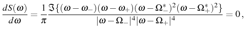Therefore, it is useful from the experimental point of view to have an analytical expression for the observed splitting that can be directly compared with the dressed modes. For this purpose, we now solve the equation $dS/d\omega=0$ , which provides the frequencies where the spectrum reaches its local extrema. There exist either one or three real solutions to this equation, corresponding to the spectrum being a singlet or a doublet, respectively. In order to compute them, we make use of the relation $dS/d\omega=\Re\{dA/d\omega\}$ , that holds thanks to the fact that $\omega \in \mathbb{R}$ . Then, the following factorization in the complex plane is possible:

$\displaystyle \frac{dS(\omega)}{d\omega}=\frac{1}{\pi}\frac{\Im\{(\omega-\omega... ...a-\Omega_+^*)^2\}}{\vert\omega-\Omega_-\vert^4\vert\omega-\Omega_+\vert^4}=0\,,$

(3.49)

with

$\displaystyle \omega_\pm=$	$\displaystyle \Big[\Omega_+-\Omega_-+iW(\Omega_++\Omega_-)\pm i\sqrt{(1+W^2)(\Omega_+-\Omega_-)^2}\Big]/2$
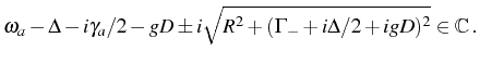
$\displaystyle =$	$\displaystyle \omega_a-\Delta-i\gamma_a/2-gD\pm i\sqrt{R^2+(\Gamma_- +i\Delta/2+igD)^2}\in\mathbb{C}\,.$	(3.50)

Despite the simple form of Eq. (3.52), none of the roots $\{\omega_{\pm},\Omega_\pm^*\}$ are its solutions, as they are not real. Actually, the solutions must be all found by taking explicitly the imaginary part in Eq. (3.52) and solving the quintic equation that this gives rise to, with coefficients too complicated to be presented here. It is well known that quintic equations cannot be solved always in terms of radicals. This happens to be our case, if we consider the most general set of parameters. The solutions can be presented, however, in terms of special functions such as the Jacobi theta functions^3.3, but such involved methods do not serve to our objective of providing clear and straight forward formulas that can be directly applied to analyze the experimental data. Therefore, in the most general case, we prefer to solve numerically Eq. (3.52), exploiting the simplicity of the equation rather than the complexity of its solutions. We will come back to these results in Sec. 3.4.3 for further and more practical discussions.

In order to give a more physical picture of the abstract results in the this one and previous Sections, we shall in the rest of this Chapter illustrate their implications in practical terms. For this purpose, we will now concentrate on the resonant case, which is the pillar of the SC physics. The main output of the out-of-resonance case is to help identify or to characterize the resonance, for instance by localizing it in an anticrossing or by providing useful additional constrains with only one more free parameter in a global fitting. Even a slight detuning brings features of WC into the SC system and ultimately, when $\vert\Delta\vert\gg g$ , the complex Rabi frequency converges into the same expression for both regimes (as showed in Fig. 3.3). This is why we now consider the SC problem in its purest form: when the coupling between the modes is optimum.