Julia programming
m |
m |
||
| Line 150: | Line 150: | ||
2 - As a phase-space solution, showing the simultaneous state of the system (here, ecosystem), with time as a parametric parameter: | 2 - As a phase-space solution, showing the simultaneous state of the system (here, ecosystem), with time as a parametric parameter: | ||
| + | psRK=plot([(yRK1[i], yRK2[i]) for i=1:npts], | ||
| + | lw=1, xlabel="x", ylabel="y", legend=false) | ||
| − | + | <center><wz tip="Phase-space solution of the Volterra-Lotka equations, still with RK4, over about 70 cycles.">[[File:Screenshot_18-03-2020_112201.jpg|400px]]</wz></center> | |
| − | < | + | |
| − | + | ||
| − | </ | + | |
This comparing the three methods together (the various plots have been evaluated as <tt>pE</tt>, <tt>pH</tt>, etc.): | This comparing the three methods together (the various plots have been evaluated as <tt>pE</tt>, <tt>pH</tt>, etc.): | ||
Revision as of 11:25, 18 March 2020
We now turn to the case of coupled equations, in which case the method reads
$$\vec y'=\vec f(t,\vec y)$$
where
$$ \vec y\equiv \begin{pmatrix} y_1\\y_2 \end{pmatrix} \quad\text{and}\quad \vec f\equiv \begin{pmatrix} f_1\\f_2 \end{pmatrix}\,. $$
The methods are the same as before just applying directly to the vectors instead. An interesting coupled system of ODE, namely, the Volterra-Lotka model of prey-predator interactions. This is modelled with the pair of coupled ODE:
\begin{align} \frac{dx}{dt} &= \alpha x - \beta x y, \\ \frac{dy}{dt} &= \delta x y - \gamma y, \end{align}
The functions are implemented as:
function f1(t,y1, y2)
    α*y1-β*y1*y2
end
function f2(t,y1, y2)
    δ*y1*y2-γ*y2
end
Some common initialization for all methods, in particular, we now need two arrays of values to store the evolution of $x$ (in y1) and $y$ (in y2):
tmax=100
h=.001
npts=round(Int,tmax/h)

y1=0.0*collect(1:npts);
y2=0.0*collect(1:npts);

y1[1]=1;
y2[1]=.1;

α=2/3;
β=4/3;
γ=1;
δ=1;
Euler's method in this case reads:
$$\vec y_{n+1}=\vec y_n+h\vec f(t_n,\vec y_n)$$
or, breaking down this equation componentwise:
$$\begin{align} y_{1,n+1}&=y_{1,n}+hf_1(t_n,y_{1,n},y_{2,n})\\ y_{2,n+1}&=y_{2,n}+hf_2(t_n,y_{1,n},y_{2,n}) \end{align}$$
In code:
@time for i=1:npts-1
    y1[i+1]=y1[i]+h*f1((i-1)*h,y1[i],y2[i])
    y2[i+1]=y2[i]+h*f2((i-1)*h,y1[i],y2[i])
end
Heun's version reads:
$$\vec y_{n+1}=\vec y_n+{h\over 2}\left(\vec f(t_n,\vec y_n)+\vec f(t_{n+1},\vec y_n+h\vec f(t_i,\vec y_n)\right)$$
or, breaking down this equation componentwise:
$$\begin{align} y_{1,n+1} &= y_{1,n} + {h\over2} [f(t_n, y_{1,n}, y_{2,n}) + f(t_n + h, y_{1,n} + h f(t_n, y_{1,n}, y_{2,n}), y_{2,n})]\\ y_{2,n+1} &= y_{2,n} + {h\over2} [f(t_n, y_{1,n}, y_{2,n}) + f(t_n + h, y_{1,n}, y_{2,n} + h f(t_n, y_{1,n}, y_{2,n}))] \end{align}$$
In code; where this time we'll find both more convenient and efficient to define auxiliary quantities, that are furthermore invoked more than once:
@time for n=1:npts-1
    tn=(n-1)*h;
    f1left=f1(tn,yH1[n],yH2[n])
    f2left=f2(tn,yH1[n],yH2[n])
    f1right=f1(tn+h,yH1[n]+h*f1left,yH2[n]+h*f2left)
    f2right=f2(tn+h,yH1[n]+h*f1left,yH2[n]+h*f2left)
    yH1[n+1]=yH1[n]+(h/2)*(f1left+f1right)
    yH2[n+1]=yH2[n]+(h/2)*(f2left+f2right)
end
RK4's version reads:
$$ \begin{align} t_{n+1} &= t_n + h\,, \\ \vec y_{n+1} &= \vec y_n + \tfrac{1}{6}\left(\vec k_1 + 2\vec k_2 + 2\vec k_3 + \vec k_4 \right)\,. \end{align} $$
in terms of the intermediate quantities:
$$ \begin{align} \vec k_1 &= h\vec f(t_n, \vec y_n)\,, \\ \vec k_2 &= h\vec f\left(t_n + \frac{h}{2}, \vec y_n + \frac{\vec k_1}{2}\right)\,, \\ \vec k_3 &= h\vec f\left(t_n + \frac{h}{2}, \vec y_n + \frac{\vec k_2}{2}\right)\,, \\ \vec k_4 &= h\vec f\left(t_n + h, \vec y_n + \vec k_3\right)\,, \end{align} $$
In code
@time for n=1:npts-1
    tn=(n-1)*h;
    # Intermediate steps
    k11=h*f1(tn,yRK1[n],yRK2[n]);
    k12=h*f2(tn,yRK1[n],yRK2[n]);
    k21=h*f1(tn+(h/2),yRK1[n]+k11/2,yRK2[n]+k12/2);
    k22=h*f2(tn+(h/2),yRK1[n]+k11/2,yRK2[n]+k12/2);
    k31=h*f1(tn+(h/2),yRK1[n]+k21/2,yRK2[n]+k22/2);
    k32=h*f2(tn+(h/2),yRK1[n]+k21/2,yRK2[n]+k22/2);
    k41=h*f1(tn+h,yRK1[n]+k31,yRK2[n]+k32);
    k42=h*f2(tn+h,yRK1[n]+k31,yRK2[n]+k32);
    # Real step
    yRK1[n+1]=yRK1[n]+(1/6)*(k11+2*k21+2*k31+k41);
    yRK2[n+1]=yRK2[n]+(1/6)*(k12+2*k22+2*k32+k42);
end
Results can be shown in two ways:
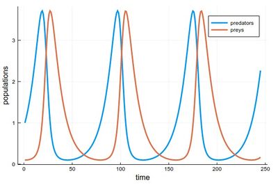
1 - As the respective solutions. This shows the oscillations of predators and preys
pRK=plot([[yRK1[i] for i=1:240], [yRK2[i] for i=1:240]],
lw=3, xlabel="time", ylabel="populations", label="RK4")

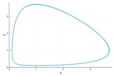
2 - As a phase-space solution, showing the simultaneous state of the system (here, ecosystem), with time as a parametric parameter:
psRK=plot([(yRK1[i], yRK2[i]) for i=1:npts], lw=1, xlabel="x", ylabel="y", legend=false)

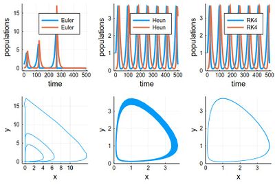
This comparing the three methods together (the various plots have been evaluated as pE, pH, etc.):
plot(pE,pH,pRK,psE,psH,psRK,layout=(2,3),dpi=150)

http://tutorial.math.lamar.edu/Classes/DE/Bernoulli.aspx
http://calculuslab.deltacollege.edu/ODE/7-C-3/7-C-3-h.html
Backward Euler method, or Implicit Euler method,