

Next: Possible extensions of this Up: Two coupled quantum dots Previous: Detrimentally symmetrical cases: Contents
Second order correlation function
In order to obtain the correlator
![]() ,
and
,
and
![]() , but also the cross correlator
, but also the cross correlator
![]() to compute
to compute
 , we can proceed as in
Sec. 3.6. Once more, the quantum
regression formula in Eq. (2.114), for the
general set of operators
, we can proceed as in
Sec. 3.6. Once more, the quantum
regression formula in Eq. (2.114), for the
general set of operators
![]() , is the same as that used to compute the mean values. We
solve the same equations, the only difference as compared with the
expressions for the LM, are the steady state vectors,
, is the same as that used to compute the mean values. We
solve the same equations, the only difference as compared with the
expressions for the LM, are the steady state vectors,
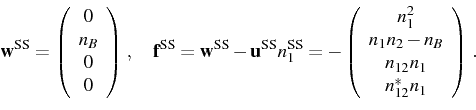
The general solutions for the correlators in the SS for
![\begin{subequations}\begin{align}&g^{(2)}(\tau)=1+\frac{[e^{-\mathbf{M}_0\tau}\,...
...bf{M}_0\tau}\,\mathbf{f}^\mathrm{SS}]_2}{n_1n_2}\, \end{align}\end{subequations}](img1268.png)
where
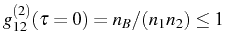 , and at infinite delay,
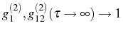 . As it
corresponds to fermions, the emission presents antibunching,
that is, the second particle cannot be emitted at the same time if it
is of the same nature as the first one, but in a posterior emission,
. As it
corresponds to fermions, the emission presents antibunching,
that is, the second particle cannot be emitted at the same time if it
is of the same nature as the first one, but in a posterior emission,
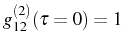 when the two dots
behave as independent. For the optimum coupling, in
Fig. 4.11,
when the two dots
behave as independent. For the optimum coupling, in
Fig. 4.11,
 can be as
small as
can be as
small as
![\includegraphics[width=0.4\linewidth]{chap4/g2/g2F.eps}](img1279.png)
![\includegraphics[width=0.4\linewidth]{chap4/g2/S2F.eps}](img1280.png) |
![\includegraphics[width=0.4\linewidth]{chap4/g2/g2c.eps}](img1283.png) |
Next: Possible extensions of this Up: Two coupled quantum dots Previous: Detrimentally symmetrical cases: Contents