

Optimally symmetrical cases:
As a first example, we study the situation where the parameters are
equal only in a crossed way:
![]() and
and
![]() . The system has a total input that is equal
to the total output,
. The system has a total input that is equal
to the total output,
![]() , and also
equal effective decoherence rates,
, and also
equal effective decoherence rates,
![]() , and,
therefore, equal Purcell rates,
, and,
therefore, equal Purcell rates, ![]() . This is a very special
situation where the symmetry is not total but exists between the
effective rates and there is a total compensation of the flows with
the exterior. It leads to
. This is a very special
situation where the symmetry is not total but exists between the
effective rates and there is a total compensation of the flows with
the exterior. It leads to
![]() and a positive
renormalization of the coupling strenght, from
and a positive
renormalization of the coupling strenght, from ![]() to
to ![]() . This is a
very unexpected effect to be completely induced by decoherence, more
precisely, by the optimal interplay between dissipation and incoherent
pump. Interestingly, the present configuration of parameters, that can
make the coupling more effective, is not accessible in the LM where
. This is a
very unexpected effect to be completely induced by decoherence, more
precisely, by the optimal interplay between dissipation and incoherent
pump. Interestingly, the present configuration of parameters, that can
make the coupling more effective, is not accessible in the LM where
![]() vanishes and the system does not have SS. In the LM,
nothing seems to indicate that the coupling gets renormalized at
resonance, decoherence has the only effect of diminishing the
splitting of the dressed states (
vanishes and the system does not have SS. In the LM,
nothing seems to indicate that the coupling gets renormalized at
resonance, decoherence has the only effect of diminishing the
splitting of the dressed states (
 ).
).
In Fig. 4.7 we have plotted the phase space
of SC as a function of
![]() and
and
![]() with the usual color code. This
configuration is in FSC only when all parameters are equal,
with the usual color code. This
configuration is in FSC only when all parameters are equal, ![]() ,
(blue line) and total symmetry is recovered. Otherwise, the
possibility of reaching all other coupling regimes opens as the
coupling is effectively improved
,
(blue line) and total symmetry is recovered. Otherwise, the
possibility of reaching all other coupling regimes opens as the
coupling is effectively improved ![]() . The SSC and MC regions are
linked to the absence of total symmetry. In the inset we can see that,
as a consequence of this special configuration, the system is richer
in spectral shapes than the ones previously studied. The lineshape can
be a doublet (area in white), a distorted doublet (light grey), a
distorted singlet (dark grey) and a singlet (black), as listed in
Table 4.1, although it never reaches a
fully formed triplet or quadruplet.
. The SSC and MC regions are
linked to the absence of total symmetry. In the inset we can see that,
as a consequence of this special configuration, the system is richer
in spectral shapes than the ones previously studied. The lineshape can
be a doublet (area in white), a distorted doublet (light grey), a
distorted singlet (dark grey) and a singlet (black), as listed in
Table 4.1, although it never reaches a
fully formed triplet or quadruplet.
![\includegraphics[width=0.7\linewidth]{chap4/examples/PS1.ps}](img1204.png) |
The ![]() -axis in Fig. 4.7, with
-axis in Fig. 4.7, with
![]() and
and
![]() , is interesting
enough with all the possible regions and lineshapes, to be analyzed in
more detail. This is the limit of maximum renormalization of the
coupling,
, is interesting
enough with all the possible regions and lineshapes, to be analyzed in
more detail. This is the limit of maximum renormalization of the
coupling,
![]() (
(
![]() ), where the populations and
mean values read
), where the populations and
mean values read
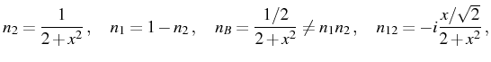
with
 . In
Fig. 4.8, we can see all these magnitudes
in the different regimes.
. In
Fig. 4.8, we can see all these magnitudes
in the different regimes.
![\includegraphics[width=0.7\linewidth]{chap4/examples/Case1.eps}](img1221.png)
![\includegraphics[width=0.45\linewidth]{chap4/examples/Case1g.eps}](img1222.png)
![\includegraphics[width=0.45\linewidth]{chap4/examples/Case1h.eps}](img1223.png) |
In the limit ![]() , there is FSC with all the levels equally
populated (
, there is FSC with all the levels equally
populated (
![]() ,
, ![]() ) and
) and
![]() . Soon
the SSC opens a bubble in the eigenenergies with the splitting of
inner and outer peaks. The transition into MC, with the collapse of
the inner peaks, takes place at
. Soon
the SSC opens a bubble in the eigenenergies with the splitting of
inner and outer peaks. The transition into MC, with the collapse of
the inner peaks, takes place at
![]() , and into WC,
closing the bubble, at
, and into WC,
closing the bubble, at
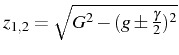
![]() . The maximum of
. The maximum of
![]() (in orange) takes place at
(in orange) takes place at ![]() , when the
coherence
, when the
coherence
![]() is maximum. This is a special point where the
splitting of the dressed mode is the largest possible,
is maximum. This is a special point where the
splitting of the dressed mode is the largest possible,
![]() ,
even though the final lineshape is a singlet. Finally, when the
coupling becomes very weak,
,
even though the final lineshape is a singlet. Finally, when the
coupling becomes very weak, ![]() , the first dot saturates and
, the first dot saturates and
![]() .
.
![\includegraphics[width=0.45\linewidth]{chap4/anticrossing/Ganticrossing.eps}](img1238.png)
![\includegraphics[width=0.45\linewidth]{chap4/anticrossing/Ganticrossing2.eps}](img1239.png)
![\includegraphics[width=0.45\linewidth]{chap4/anticrossing/Hanticrossing.eps}](img1240.png)
![\includegraphics[width=0.45\linewidth]{chap4/anticrossing/Hanticrossing2.eps}](img1241.png) |
The spectra acquire interesting lineshapes: a doublet in SSC that gets
distorted due to the underlying quadruplet structure, in
Fig. 4.8(g), and then a singlet distorted
due to the underlying triplet structure, in (h), as the two inner
peaks stick together. Before reaching WC, the spectra has become a
plain singlet. The way to distinguish mathematically the different
possible shapes is explained in
Table 4.1. The anticrossing that this
lineshapes form when detuning between the modes is varied from zero to
![]() , is also peculiar. In
Fig. 4.9(a) and (d) we can see that the
distorted doublet and singlet (resp.) keep their features up to
, is also peculiar. In
Fig. 4.9(a) and (d) we can see that the
distorted doublet and singlet (resp.) keep their features up to
![]() and
and
![]() (resp.). Note
that the singlet maxima oscillates around the origin: first, to the
left, then, right and finally center, when the detuning is larger than
in the plot. In all cases, the emission at
(resp.). Note
that the singlet maxima oscillates around the origin: first, to the
left, then, right and finally center, when the detuning is larger than
in the plot. In all cases, the emission at
![]() is dominant
over
is dominant
over
![]() because the first dot is being pumped and
the second dissipates the excitation. The underlying structure is
plotted next to them, in (b) and (d), showing the profile of the four
and three peaks that form the spectra.
because the first dot is being pumped and
the second dissipates the excitation. The underlying structure is
plotted next to them, in (b) and (d), showing the profile of the four
and three peaks that form the spectra.
Elena del Valle ©2009-2010-2011-2012.