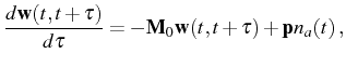
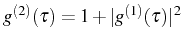
Second order correlation function
The correlator
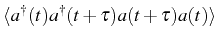 needed to
compute
needed to
compute
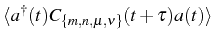
 , requires to apply the quantum regression
formula in Eq. (2.114) for the general set
of operators
, requires to apply the quantum regression
formula in Eq. (2.114) for the general set
of operators
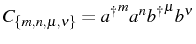 (that
includes
(that
includes  ) with
 and
and
 . As we
noted in Sec. 2.7, the quantum regression
formula is the same as that used to compute the mean values of
Sec. 3.2. The set of correlators
. As we
noted in Sec. 2.7, the quantum regression
formula is the same as that used to compute the mean values of
Sec. 3.2. The set of correlators
 is again reduced to
 (see
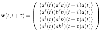
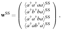
Fig. 3.2). We write explicitly these four
correlators, linked to
(see
Fig. 3.2). We write explicitly these four
correlators, linked to
 , in the form
 and construct the
vector
and construct the
vector
 |
(3.73) |
The equation we must solve reads
 |
(3.74) |
with the same matrix

and pumping vector

[Eqs. (
3.7a)] that already appeared in
Eq. (
3.6) for the mean values. If we concentrate on the SS
case, the initial conditions

are given by the SS
values,
 |
(3.75) |
and

. These new four average
quantities can be obtained by applying once more the quantum
regression formula, in the same way we did to obtain

, having in mind the schema on the right of
Fig.
3.2. However, the quantities in

correspond to

in the
second manifold,

(not plotted
in Fig.
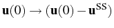
3.2). We need to obtain all
correlators in

:
The new set of equations link these elements among themselves and to
those in the first manifold, that we already computed. Now that we
know how to obtain
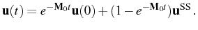
, we can write the solution
of Eq. (3.77) as:
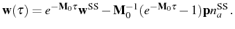 |
(3.77) |
Remembering from Sec. 3.2 that
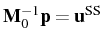 , the solution can
be further simplified into:
, the solution can
be further simplified into:
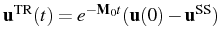
 |
(3.78) |
If we define the SS fluctuation vector,
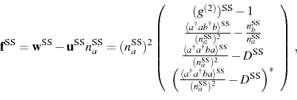 |
|
|
(3.79) |
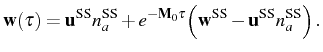
we can write a general expression for
(with  ):
):
![$\displaystyle g^{(2)}(\tau)=\frac{[\mathbf{w}(\tau)]_1}{(n_a^\mathrm{SS})^2}=1+\frac{[e^{-\mathbf{M}_0\tau}\,\mathbf{f}^\mathrm{SS}]_1}{(n_a^\mathrm{SS})^2}\,,$](img962.png) |
(3.80) |
where
![$ [\mathbf{x}]_1$](img963.png) means that we take the first element of the
vector
means that we take the first element of the
vector
 . Note that for the present system,
 and
and
 |
(3.81) |
A more explicit expression of
in terms of the system
parameters, can be obtained by analogy with the solution for
 in Eq. (3.9),
by exchanging
in Eq. (3.9),
by exchanging  for
for  and the elements in
 for
those in
for
those in
 . However,
can be more straightforwardly obtained from the
relation
. However,
can be more straightforwardly obtained from the
relation
 , that applies for thermal
photons (Eq. 2.115). Two emission events are
independent from each other in this case, where we also have
, that applies for thermal
photons (Eq. 2.115). Two emission events are
independent from each other in this case, where we also have
 . For the sake of completeness, we
can write the explicit expressions in the SS for
and
. For the sake of completeness, we
can write the explicit expressions in the SS for
and
 :
with the definitions of Eq. (3.39) and
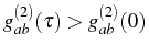
(3.12). As it corresponds to bosons, the
emission presents bunching, that is, the second photon prefers
to be emitted together with the first one,
:
with the definitions of Eq. (3.39) and
(3.12). As it corresponds to bosons, the
emission presents bunching, that is, the second photon prefers
to be emitted together with the first one,
 .
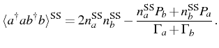
The SS
goes from its zero delay value,
.
The SS
goes from its zero delay value,  , towards
the infinite delay value,
, towards
the infinite delay value,  , with damped oscillations in SC [see
Fig. 3.18(a) in solid blue] and exponential
decay in the WC. In all cases, the transient in happens at
twice the speed of
, with damped oscillations in SC [see
Fig. 3.18(a) in solid blue] and exponential
decay in the WC. In all cases, the transient in happens at
twice the speed of
 , given also in terms of
  and
and
 . The noise spectrum in SC consists of three peaks, one
centered at zero and the other two at
. The noise spectrum in SC consists of three peaks, one
centered at zero and the other two at
 [see
Fig. 3.18(b)].
[see
Fig. 3.18(b)].
Another correlator of interest is the cross second order correlation
function,
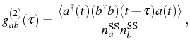 |
(3.83) |
a quantity related with the probability of emitting an exciton (direct
emission) at after having emitted a photon and  . This is
computed together with the
:
. This is
computed together with the
:
![$\displaystyle g_{ab}^{(2)}(\tau)=\frac{[\mathbf{w}(\tau)]_2}{n_a^{\mathrm{SS}} ...
...M}_0\tau}\,\mathbf{f}^{\mathrm{SS}}]_2}{n_a^{\mathrm{SS}} n_b^{\mathrm{SS}}}\,.$](img981.png) |
(3.84) |
In this case, the correlator goes from
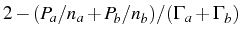 to [see
Fig. 3.18(a) in dashed purple]. The zero
delay value is not in general. It is exactly only when
to [see
Fig. 3.18(a) in dashed purple]. The zero
delay value is not in general. It is exactly only when
 , and the modes behave as if they
were independent
with
, and the modes behave as if they
were independent
with
 . One
case is the very WC, with the modes really independent, and the other
one, is the very SC, where excitation is equally shared between the
modes as
. One
case is the very WC, with the modes really independent, and the other
one, is the very SC, where excitation is equally shared between the
modes as
 . However
these two cases are clearly distinguished in the rest of the
dynamics. In the very SC, the oscillations of
. However
these two cases are clearly distinguished in the rest of the
dynamics. In the very SC, the oscillations of
 reach alternating exactly with
. In the most
general case,
can have starting values between
and , as in Fig. 3.19. In their SC
experiments, Hennessy et al. (2007) computed this kind of cross
two-photon counting for large detuning, where the cavity and excitonic
modes can be clearly resolved separately. Contrary to our present
case, they observed antibunching with
reach alternating exactly with
. In the most
general case,
can have starting values between
and , as in Fig. 3.19. In their SC
experiments, Hennessy et al. (2007) computed this kind of cross
two-photon counting for large detuning, where the cavity and excitonic
modes can be clearly resolved separately. Contrary to our present
case, they observed antibunching with
 , demonstrating that the modes are
coupled and that the QD is not bosonic.
, demonstrating that the modes are
coupled and that the QD is not bosonic.
The full dynamics of the general one-time average values in
 , that we computed in
Sec. 3.2 only for the SS or in the absence
of pump, can be obtained now with no additional effort by simple analogy with
Eq. (3.81):
, that we computed in
Sec. 3.2 only for the SS or in the absence
of pump, can be obtained now with no additional effort by simple analogy with
Eq. (3.81):
 |
(3.85) |
The transient part of the dynamics,
 ,
has the same mathematical expression as
,
making the substitutions (
,
has the same mathematical expression as
,
making the substitutions (
 ),
(
),
(
 ) and
) and
 . Therefore, the
frequency/damping of the oscillations in the transient is also given
by real/imaginary part of .
. Therefore, the
frequency/damping of the oscillations in the transient is also given
by real/imaginary part of .
Elena del Valle
©2009-2010-2011-2012.


![\begin{subequations}\begin{align}&g^{(2)}(\tau)=1+e^{-2\Gamma_+\tau}\Big\{ \frac...
...2R_\mathrm{i})^2+(\omega-2R_\mathrm{r})^2}\Big]\,, \end{align}\end{subequations}](img971.png)
![\includegraphics[width=0.45\linewidth]{chap3/g2/g2.eps}](img978.png)
![\includegraphics[width=0.45\linewidth]{chap3/g2/S2.eps}](img979.png)
![\includegraphics[width=0.45\linewidth]{chap3/g2/g2c.eps}](img988.png)