Crash Course in Scientific Computing
7. Algorithms: the idea
«An algorithm must be seen to be believed.»—Donald Knuth, TAOCP Vol. I, Fundamental Algorithms
An algorithm is a recipe to solve a problem with a computer, a list of instructions for the later to follow that will bring it to the solution, which it can duly report. Problems are of all types, from scientific problems such as finding roots of complex functions to integrating differential equations passing by everybody's daily problems such as finding the shortest or best route to bring you from A to B in a complex map or sorting the list of top results in an internet query. The set of instructions can be efficient and lead to a rapid, accurate and faithful solution from the computer, or on the opposite, clumsy, redundant and leading it to waste resources and possibly not even the best, or a good, or even any solution at all. The art of finding a good algorithm has been guiding scientists and engineers since antiquity. Any single problem typically comes with a myriad of different algorithms. For many problems, such as integer factorization, we do not have yet, and probably will never have, good algorithms which can perform the job in a reasonable time. This problem has actually been turned into an opportunity, to form the basis for today's cryptography: multiplying two large numbers is easy, factoring out back their product is difficult. One can show (next lecture) how to encode messages from this asymmetry.
One of the simplest algorithms is to find the largest number in a list that has no particular order. We will use this as a starting point to illustrate the above concepts. It is a simple algorithm because its best implementation is basically what one would do anyway: go through each element in turn, if the element we currently examine is larger than the largest we found so far, we update our record, if not, we carry on. Here's a Julia implementation:
function myfindmax(lst)
    i=1;
    imax=length(lst);
    lmax=lst[1]
    while i<imax
    i+=1;
        if lst[i]>lmax
            lmax=lst[i]
        end
    end
    lmax
end
Example application, how close do we get from 1 in 10 random trials?
julia> myfindmax(rand(10))
0.985052934036265
Although in principle it is better to test your algorithm on cases which you know and that you can check yourself by hand:
julia> known=rand(Int8, 5)
5-element Array{Int8,1}:
 -13
 -94
  22
  90
 -86

julia> myfindmax(known)
90

julia> myfindmax(abs.(known))
94
It is also good to test on particular as well as extreme cases, e.g., when the max element is first or last. For instance, if we would have specified the increment i+=1 after the test, the algorithm would fail if the max would find itself as the last element of the array (which would be the case if the list would be ordered):
julia> myfindmax([i for i=1:10])
10
An important aspect of algorithms is their efficiency, how fast and good they are in performing the job. To benchmark, one can use @time or, if wanting to store the result for later processing, @elapsed (!!):
julia> mytime=zeros(100);
julia> for i=1:100
           lst = rand(10^6)
           mytime[i] = @elapsed myfindmax(lst);
       end

julia> comptime=zeros(100);
julia> for i=1:100
           lst = rand(10^6)
           comptime[i] = @elapsed maximum(lst);
       end

julia> plot([mytime comptime], label=["us" "julia"], xlabel="Run", ylabel="Time (s)")
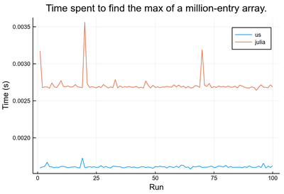
As an exception to the general rule, we find here that our own implementation is actually faster than the one provided by the system:
julia> mean(mytime)
0.0016102164000000002

julia> mean(comptime)
0.0027113203900000003
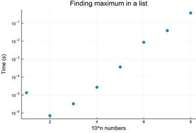
The "complexity" of our find-max algorithm is linear: it grows in direct proportion to the size of the input, as can be understood easily from the way the algorithm is designed. Here is this relationship explictely calculated by the computer:
julia>  lt=[@elapsed myfindmax(rand(10^i)) for i=1:8]
julia> scatter(lt, yscale=:log10, xlabel="10^n numbers", ylabel="Time (s)",
 title="Finding maximum in a list", legend=false)
To do even more advanced benchmarking, one can be
julia> using BenchmarkTools
julia> @benchmark myfindmax(rand(10^6))
BenchmarkTools.Trial:
  memory estimate:  7.63 MiB
  allocs estimate:  2
  --------------
  minimum time:     2.015 ms (0.00% GC)
  median time:      2.061 ms (0.00% GC)
  mean time:        2.184 ms (4.24% GC)
  maximum time:     42.876 ms (88.56% GC)
  --------------
  samples:          2285
  evals/sample:     1

julia> @benchmark maximum(rand(10^6))
BenchmarkTools.Trial:
  memory estimate:  7.63 MiB
  allocs estimate:  2
  --------------
  minimum time:     3.344 ms (0.00% GC)
  median time:      3.461 ms (0.00% GC)
  mean time:        3.570 ms (3.05% GC)
  maximum time:     44.792 ms (91.19% GC)
  --------------
  samples:          1399
  evals/sample:     1
The fact that our readily-made version is faster than the one provided by the system has been flagged by the Julia community and has been traced to time being lost when checking for NaN numbers.
Algorithms usually rely on tricks or clever observations. For instance, whatever the numbers $y$ and $x$, it is always true that $\sqrt{x}$ is comprised between $y$ and $x/y$. This is easy to prove and follow from the fact that $1/\sqrt{x}=\sqrt{x}/x$. If $y<\sqrt{x}$, then $1/y>\sqrt{x}/x$ which brings us to
$$y<\sqrt{x}<x/y$$
while if $y>\sqrt{x}$ then, similarly, $1/y<\sqrt{x}/x$ and we have the opposite inequality
$$x/y<\sqrt{x}<y$$
So given to numbers $x$ and $y$, a good guess to approximate $\sqrt{x}$ is to take their average ${1\over2}(y+x/y)$. We now have a number closer to $\sqrt{x}$, so we can simply iterate. This is, thus, our algorithm, start with any $y_0\neq x$ and compute:
$$y_{n+1}={1\over2}\left(y_n+{x\over y_n}\right)$$
This will converge to $\sqrt{x}$. This method was known to the Babylonians to compute $\sqrt{2}$. This is the Julia code:
julia> x=2; y=1;
julia> while abs(y^2-x)>10^-12
           global y=(1/2)*(y+x/y)
           println(y)
       end
1.5
1.4166666666666665
1.4142156862745097
1.4142135623746899
1.414213562373095

julia> √2
1.4142135623730951
This is frustratingly fast! Numerical analysis shows that the number of significant digits doubles at each step. We don't need any better algorithm than this one designed by the Babylonians, and this is actually the steps that are undertaken by your pocket calculator, or any computer for that matter, when you press the √ button. Wherever it starts from, in just a few steps, it will have all the decimals of its accuracy correct to the sought square root So now you how this happens.
We are limited by machine precision when running such algorithms. Show that using big numbers, you get $\sqrt{2}$ as:
1.414213562373095048801688724209698078569671875376948073176679737990732478462119
What does it tell you about the previous approximation? How many steps did it take to bring you there? Explore the case using exact fractions with x=2//1 and y=1//1.
In fact, many efficient algorithms for such important problems originate from very ancient times. Let us see the implementations for some of them, starting with those numbers at the heart of number theory, namely, primes, i.e., those numbers which only have themselves and 1 as possible divisors. This also comes back from antiquity, namely, from Eratosthenes who proposed the following algorithm:
- Arrange numbers in a list.
- Start at 2 (1 is an exception).
- Cross out all the multiples of 2 in the table.
- Proceed to the next number which has not been crossed out.
- Cross out all the multiples of this number in the table.
- Return to step 4 until you reach the end of the table.
- The numbers which are left is an ordered list of primes numbers up to the size of your table.
This is an implementation in Julia: we will work with BitArray to optimize space, where each entry of the array is either 1 (true) or 0 (false), depending on whether the number with this index is prime or not. Let's work up to 2500 (a perfect square so we can draw our result). Calling erato this array and remembering that 1 is not prime:
nmax=50*50
erato=trues(nmax);
erato[1]=false;
we can cross-out numbers through Eratosthenes' sieve as follows:
for i∈2:nmax
    if erato[i]
        erato[i*(i:nmax÷i)].=0
    end
end
We now have an array of true at the positions of numbers that survived the sieving, i.e., which are not multiple of any other number except 1 and themselves, i.e., prime numbers. We can retrieve these numbers as follows:
lprimes=findall(p->(p==true), erato)
Here is a graph of the prime distributions up to 2500 (using our plotspace function from our plotting Lecture):
plotspace(reshape(erato,50,50))
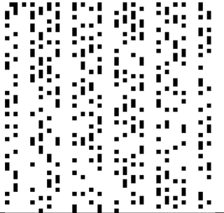
We will leave it there although there has been enthusiastic activity in chasing patterns in such plots, most famously with Ulam's spiral.
We could check this result with julia's facilities to test for primality, which are found in
using Primes
This is checking that all numbers in our list are primes:
julia> unique(isprime.(lprimes))
1-element Array{Bool,1}:
 true
but this is not checking that we found all the primes. One way to do it is to check that we have the same number of elements:
julia> counter=0;

julia> for i∈1:nmax
           if isprime(i)
               global counter+=1
           end
       end

julia> counter
367

julia> length(lprimes)
367
So the result is correct, up to 5000. We can now look at the prime-counting function $\pi(x)$ that counts how many primes there are below $x$:
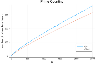
Gauss approximated $\pi(x)$ by $x/\ln(x)$ when he was only 15. There has been, subsequently, several improvements, including from Legendre who introduced an eponymous constant to fit this function. We let you play with higher numbers.
Find the largest prime below $10^9$ and which number is it in the list of primes? Which one is next? How does this compare to Gauss' approximation?
Answer: This is $999\,999\,937$, the $50\,847\,534$th prime number, for which the prime-counting function $\pi(x)$ compares to Gauss' approximation $\pi(x)\approx x/\ln x=48\,254\,942$ to withing 5% accuracy. The next prime is $1\,000\,000\,007$.
Another very important algorithm is the so-called Euclidean algorithm to perform Euclidean—or integer—division. This takes two (positive, without loss of generality) integers $a$ (numerator) and $b$ (denominator) and returns another two integers: $q$ (quotient) and $r$ (remainder)
$$a=bq+r$$
with $0\le q<p$. We have seen that julia computes these quantities directly so there is no need of an algorithm per se:
julia> function juliadiv(a,b)
           [a÷b, a%b]
       end
but to know what's inside the box, let us look at various implementations. The oldest one is from Euclid himself, in his Elements, Book VII, Proposition 1, a simple method is proposed: starting with $r=a$, while $r\ge b$, subtract $b$ from $r$ and take this as the new $r$ and when this is not possible, what is left is the final remainder $r$. The number of times it took to get there is $q$. In julia code:
function eucliddiv(a,b)
    r=a
    q=0
    while r-b ≥ 0
        q+=1
        r=r-b
    end
    [q r]
end
This is very simple but can get quite lengthy. One would use long division algorithms for faster results. Instead of looking at those now, we turn to an important historical algorithm, Euclid's algorithm, which computes the gcd (greatest common divisor between two numbers). This is one of the oldest known algorithms. It is based one the fact that the gcd of two numbers is the same as the gcd of the smaller number with the positive difference of the numbers, so that by iterations, one can decrease the values of the numbers until they become equal, at which point the value thus found is the gcd. This is a julia implementation:
function euclidgcd(a,b)
    while a!=b
        if a > b
            a = a-b
        elseif a < b
            b = b-a
        end
    end
    a
end
This is the result, showing the details of the intermediate steps:
function euclidgcd(a,b)
    i=0;
    while a!=b
        if a > b
            a = a-b
        elseif a < b
            b = b-a
        end
        i+=1;
        println("step $(i):  a=$(a) b=$(b)")
    end
    a
end
julia> a=abs(rand(Int))
3371149190952905360

julia> b=4884762153376862325
4884762153376862325

step 1:  a=3371149190952905360 b=1513612962423956965
step 2:  a=1857536228528948395 b=1513612962423956965
step 3:  a=343923266104991430 b=1513612962423956965
step 4:  a=343923266104991430 b=1169689696318965535
step 5:  a=343923266104991430 b=825766430213974105
step 6:  a=343923266104991430 b=481843164108982675
step 7:  a=343923266104991430 b=137919898003991245
step 8:  a=206003368101000185 b=137919898003991245
step 9:  a=68083470097008940 b=137919898003991245
step 10:  a=68083470097008940 b=69836427906982305
step 11:  a=68083470097008940 b=1752957809973365
step 12:  a=66330512287035575 b=1752957809973365
step 13:  a=64577554477062210 b=1752957809973365
step 14:  a=62824596667088845 b=1752957809973365
step 15:  a=61071638857115480 b=1752957809973365
step 16:  a=59318681047142115 b=1752957809973365
step 17:  a=57565723237168750 b=1752957809973365
step 18:  a=55812765427195385 b=1752957809973365
step 19:  a=54059807617222020 b=1752957809973365
step 20:  a=52306849807248655 b=1752957809973365
step 21:  a=50553891997275290 b=1752957809973365
step 22:  a=48800934187301925 b=1752957809973365
step 23:  a=47047976377328560 b=1752957809973365
step 24:  a=45295018567355195 b=1752957809973365
step 25:  a=43542060757381830 b=1752957809973365
step 26:  a=41789102947408465 b=1752957809973365
step 27:  a=40036145137435100 b=1752957809973365
step 28:  a=38283187327461735 b=1752957809973365
step 29:  a=36530229517488370 b=1752957809973365
step 30:  a=34777271707515005 b=1752957809973365
step 31:  a=33024313897541640 b=1752957809973365
step 32:  a=31271356087568275 b=1752957809973365
step 33:  a=29518398277594910 b=1752957809973365
step 34:  a=27765440467621545 b=1752957809973365
step 35:  a=26012482657648180 b=1752957809973365
step 36:  a=24259524847674815 b=1752957809973365
step 37:  a=22506567037701450 b=1752957809973365
step 38:  a=20753609227728085 b=1752957809973365
step 39:  a=19000651417754720 b=1752957809973365
step 40:  a=17247693607781355 b=1752957809973365
step 41:  a=15494735797807990 b=1752957809973365
step 42:  a=13741777987834625 b=1752957809973365
step 43:  a=11988820177861260 b=1752957809973365
step 44:  a=10235862367887895 b=1752957809973365
step 45:  a=8482904557914530 b=1752957809973365
step 46:  a=6729946747941165 b=1752957809973365
step 47:  a=4976988937967800 b=1752957809973365
step 48:  a=3224031127994435 b=1752957809973365
step 49:  a=1471073318021070 b=1752957809973365
step 50:  a=1471073318021070 b=281884491952295
step 51:  a=1189188826068775 b=281884491952295
step 52:  a=907304334116480 b=281884491952295
step 53:  a=625419842164185 b=281884491952295
step 54:  a=343535350211890 b=281884491952295
step 55:  a=61650858259595 b=281884491952295
step 56:  a=61650858259595 b=220233633692700
step 57:  a=61650858259595 b=158582775433105
step 58:  a=61650858259595 b=96931917173510
step 59:  a=61650858259595 b=35281058913915
step 60:  a=26369799345680 b=35281058913915
step 61:  a=26369799345680 b=8911259568235
step 62:  a=17458539777445 b=8911259568235
step 63:  a=8547280209210 b=8911259568235
step 64:  a=8547280209210 b=363979359025
step 65:  a=8183300850185 b=363979359025
step 66:  a=7819321491160 b=363979359025
step 67:  a=7455342132135 b=363979359025
step 68:  a=7091362773110 b=363979359025
step 69:  a=6727383414085 b=363979359025
step 70:  a=6363404055060 b=363979359025
step 71:  a=5999424696035 b=363979359025
step 72:  a=5635445337010 b=363979359025
step 73:  a=5271465977985 b=363979359025
step 74:  a=4907486618960 b=363979359025
step 75:  a=4543507259935 b=363979359025
step 76:  a=4179527900910 b=363979359025
step 77:  a=3815548541885 b=363979359025
step 78:  a=3451569182860 b=363979359025
step 79:  a=3087589823835 b=363979359025
step 80:  a=2723610464810 b=363979359025
step 81:  a=2359631105785 b=363979359025
step 82:  a=1995651746760 b=363979359025
step 83:  a=1631672387735 b=363979359025
step 84:  a=1267693028710 b=363979359025
step 85:  a=903713669685 b=363979359025
step 86:  a=539734310660 b=363979359025
step 87:  a=175754951635 b=363979359025
step 88:  a=175754951635 b=188224407390
step 89:  a=175754951635 b=12469455755
step 90:  a=163285495880 b=12469455755
step 91:  a=150816040125 b=12469455755
step 92:  a=138346584370 b=12469455755
step 93:  a=125877128615 b=12469455755
step 94:  a=113407672860 b=12469455755
step 95:  a=100938217105 b=12469455755
step 96:  a=88468761350 b=12469455755
step 97:  a=75999305595 b=12469455755
step 98:  a=63529849840 b=12469455755
step 99:  a=51060394085 b=12469455755
step 100:  a=38590938330 b=12469455755
step 101:  a=26121482575 b=12469455755
step 102:  a=13652026820 b=12469455755
step 103:  a=1182571065 b=12469455755
step 104:  a=1182571065 b=11286884690
step 105:  a=1182571065 b=10104313625
step 106:  a=1182571065 b=8921742560
step 107:  a=1182571065 b=7739171495
step 108:  a=1182571065 b=6556600430
step 109:  a=1182571065 b=5374029365
step 110:  a=1182571065 b=4191458300
step 111:  a=1182571065 b=3008887235
step 112:  a=1182571065 b=1826316170
step 113:  a=1182571065 b=643745105
step 114:  a=538825960 b=643745105
step 115:  a=538825960 b=104919145
step 116:  a=433906815 b=104919145
step 117:  a=328987670 b=104919145
step 118:  a=224068525 b=104919145
step 119:  a=119149380 b=104919145
step 120:  a=14230235 b=104919145
step 121:  a=14230235 b=90688910
step 122:  a=14230235 b=76458675
step 123:  a=14230235 b=62228440
step 124:  a=14230235 b=47998205
step 125:  a=14230235 b=33767970
step 126:  a=14230235 b=19537735
step 127:  a=14230235 b=5307500
step 128:  a=8922735 b=5307500
step 129:  a=3615235 b=5307500
step 130:  a=3615235 b=1692265
step 131:  a=1922970 b=1692265
step 132:  a=230705 b=1692265
step 133:  a=230705 b=1461560
step 134:  a=230705 b=1230855
step 135:  a=230705 b=1000150
step 136:  a=230705 b=769445
step 137:  a=230705 b=538740
step 138:  a=230705 b=308035
step 139:  a=230705 b=77330
step 140:  a=153375 b=77330
step 141:  a=76045 b=77330
step 142:  a=76045 b=1285
step 143:  a=74760 b=1285
step 144:  a=73475 b=1285
step 145:  a=72190 b=1285
step 146:  a=70905 b=1285
step 147:  a=69620 b=1285
step 148:  a=68335 b=1285
step 149:  a=67050 b=1285
step 150:  a=65765 b=1285
step 151:  a=64480 b=1285
step 152:  a=63195 b=1285
step 153:  a=61910 b=1285
step 154:  a=60625 b=1285
step 155:  a=59340 b=1285
step 156:  a=58055 b=1285
step 157:  a=56770 b=1285
step 158:  a=55485 b=1285
step 159:  a=54200 b=1285
step 160:  a=52915 b=1285
step 161:  a=51630 b=1285
step 162:  a=50345 b=1285
step 163:  a=49060 b=1285
step 164:  a=47775 b=1285
step 165:  a=46490 b=1285
step 166:  a=45205 b=1285
step 167:  a=43920 b=1285
step 168:  a=42635 b=1285
step 169:  a=41350 b=1285
step 170:  a=40065 b=1285
step 171:  a=38780 b=1285
step 172:  a=37495 b=1285
step 173:  a=36210 b=1285
step 174:  a=34925 b=1285
step 175:  a=33640 b=1285
step 176:  a=32355 b=1285
step 177:  a=31070 b=1285
step 178:  a=29785 b=1285
step 179:  a=28500 b=1285
step 180:  a=27215 b=1285
step 181:  a=25930 b=1285
step 182:  a=24645 b=1285
step 183:  a=23360 b=1285
step 184:  a=22075 b=1285
step 185:  a=20790 b=1285
step 186:  a=19505 b=1285
step 187:  a=18220 b=1285
step 188:  a=16935 b=1285
step 189:  a=15650 b=1285
step 190:  a=14365 b=1285
step 191:  a=13080 b=1285
step 192:  a=11795 b=1285
step 193:  a=10510 b=1285
step 194:  a=9225 b=1285
step 195:  a=7940 b=1285
step 196:  a=6655 b=1285
step 197:  a=5370 b=1285
step 198:  a=4085 b=1285
step 199:  a=2800 b=1285
step 200:  a=1515 b=1285
step 201:  a=230 b=1285
step 202:  a=230 b=1055
step 203:  a=230 b=825
step 204:  a=230 b=595
step 205:  a=230 b=365
step 206:  a=230 b=135
step 207:  a=95 b=135
step 208:  a=95 b=40
step 209:  a=55 b=40
step 210:  a=15 b=40
step 211:  a=15 b=25
step 212:  a=15 b=10
step 213:  a=5 b=10
step 214:  a=5 b=5
5
This goes reasonably fast, but still requires a lot of steps... Instead of the difference, one can replace the smaller number by the remainder of Euclidean division of the larger number by the smaller one. In this way, our algorithm improves to:
function euclidlamegcd(a,b)
    i=0;
    while min(a,b)!=0
        if a > b
            a = a%b
        elseif a < b
            b = b%a
        end
    i+=1;
    println("step $(i):  a=$(a) b=$(b)")
    end
    max(a,b)
end
and indeed this is much "faster":
julia> euclidlamegcd(a,b)
step 1:  a=3371149190952905360 b=1513612962423956965
step 2:  a=343923266104991430 b=1513612962423956965
step 3:  a=343923266104991430 b=137919898003991245
step 4:  a=68083470097008940 b=137919898003991245
step 5:  a=68083470097008940 b=1752957809973365
step 6:  a=1471073318021070 b=1752957809973365
step 7:  a=1471073318021070 b=281884491952295
step 8:  a=61650858259595 b=281884491952295
step 9:  a=61650858259595 b=35281058913915
step 10:  a=26369799345680 b=35281058913915
step 11:  a=26369799345680 b=8911259568235
step 12:  a=8547280209210 b=8911259568235
step 13:  a=8547280209210 b=363979359025
step 14:  a=175754951635 b=363979359025
step 15:  a=175754951635 b=12469455755
step 16:  a=1182571065 b=12469455755
step 17:  a=1182571065 b=643745105
step 18:  a=538825960 b=643745105
step 19:  a=538825960 b=104919145
step 20:  a=14230235 b=104919145
step 21:  a=14230235 b=5307500
step 22:  a=3615235 b=5307500
step 23:  a=3615235 b=1692265
step 24:  a=230705 b=1692265
step 25:  a=230705 b=77330
step 26:  a=76045 b=77330
step 27:  a=76045 b=1285
step 28:  a=230 b=1285
step 29:  a=230 b=135
step 30:  a=95 b=135
step 31:  a=95 b=40
step 32:  a=15 b=40
step 33:  a=15 b=10
step 34:  a=5 b=10
step 35:  a=5 b=0
5
The improvement from Euclid's method to the gcd makes the algorithm require a number of steps which is at most five times the number of digits (in base 10) of the smaller integer. This was proven by Gabriel Lamé in 1844 and marks the beginning of computational complexity theory. There has been indeed many studies in general and optimizations in particular of this simple algorithm, which turns out to have many applications in number theory. We will conclude this first overview of algorithms by a typical implementation of Euclidean's algorithm in native computer language, namely, using binary representation, in which case multiplications can be turned to binary shift and other peculiarities of this base can be taken advantage of (we have seen for instance how floats can have a precision of 53 bits with 52 bits only).
function euclidsteingcd(a,b)
    println("$(a) $(b)")
    if a==b
        a
    elseif a==1 || b==1
        1
    elseif iseven(a)
        if iseven(b)
            2*euclidsteingcd(a>>1, b>>1)
        else
            euclidsteingcd(a>>1, b)
        end
    elseif iseven(b)
        euclidsteingcd(a, b>>1)
    else
        euclidsteingcd(abs(a-b)>>1, min(a,b))
    end
end
Check that the probability for two integers taken randomly to have no common factor is given by $6/\pi^2$ [1].
This will check it numerically for a billion points using the various methods that we have implemented as compared to the native method and the exact result, sorted in reverse-order of their efficiency:
julia> @time sum([euclidgcd(abs(rand(Int)),abs(rand(Int)))==1 for i=1:10^9])/10^9
1201.278131 seconds (63.59 k allocations: 956.771 MiB, 0.01% gc time)
0.607893579

julia> @time sum([euclidsteingcd(abs(rand(Int)),abs(rand(Int)))==1 for i=1:10^9])/10^9
598.468639 seconds (80.59 k allocations: 957.648 MiB, 0.00% gc time)
0.607916308

julia> @time sum([euclidlamegcd(abs(rand(Int)),abs(rand(Int)))==1 for i=1:10^9])/10^9
427.323065 seconds (62.87 k allocations: 956.742 MiB, 0.04% gc time)
0.607932819

julia> @time sum([gcd(abs(rand(Int)),abs(rand(Int)))==1 for i=1:10^9])/10^9
226.379316 seconds (68.10 k allocations: 956.948 MiB, 0.04% gc time)
0.607926964

julia> 6/pi^2
0.6079271018540267
The Stein algorithm is supposed to be very fast but our implementation turns out to be significantly less efficient than Lamé's simple improvement (algorithmically) over Euclid's version. Maybe we did not take full advantage of its enhancement. The problem we have is that this still requires a huge number of steps as reducing the numbers is done by substraction of the minimum number. The gain of only using multiplication and division do not compensate for that, if at all. This would require further analysis. The fact that the fastest method also seem to be more accurate is, however, completely by chance!
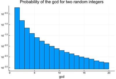
Here is the distribution of possible common factors:
julia> histogram([euclidlamegcd(abs(rand(Int)),abs(rand(Int))) for i=1:10^6],bins=1:20,yscale=:log10,
       legend=false,xlabel="gcd",norm=true,title="Probability of the gcd for two random integers")
Much of the rest of the course will in implementing such numerical algorithms, to tackle mathematical questions. In fact, the name "algorithm" itself comes from Muḥammad ibn Mūsā al-Khwārizmī, whom we already met in our Mathematics lectures when discussing algebra. We will see in particular how to find roots of nonlinear equations, differentiate and integrate, interpolate and extrapolate, solve differential equations, etc., but it would wrong to reduce algorithms and computer science to mathematical tasks of this type. In fact, we shall devote the next lecture to particular non-mathematical algorithms that Physicists should know about, because their tasks relate to physical concepts, or simply due to their importance.