Computación I: Data Fitting
Fitting out of the box
We have witnessed already the natural appearance of the Normal distribution and we used a formula to estimate its standard deviation.
Another way would be to explicit fit the data. Like this, we can also see if the data is actually normally distributed!
Like many software, matlab comes with buil-in tools to fit data. This is powerful, but power demands responsibility, and unless one knows what one is doing, such black-box approaches are typically slippery.
Let us try anyway as if there is no tomorrow. We thus generate data again, namely, the average of $n$ random numbers (uniformly distributed). This below is the case for $n=10$ (calling the variable sampleSize):
numpts=10000; % number of data points we will deal with
sampleSize=10; % number of random numbers we average

data=zeros(numpts,1); % pre-allocation

for i=1:numpts
    data(i)=mean(rand(sampleSize,1));
end

dx=0.01;
partition = [0:dx:1];

distribution = histcounts(data,partition,'Normalization', 'probability')/dx;
x=linspace(0,1,length(distribution));

xlabel('mean');
ylabel('probability');

gaussian='exp(-(x-x0).^2/(2*sx^2))/(sqrt(2*pi*sx^2))'

%f=fit(x',distribution',gaussian)
f=fit(x',distribution',gaussian,'Start',[0.5 0.5])

plot(f,x,distribution)
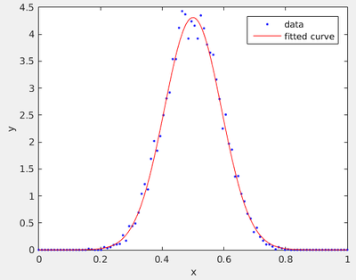
We put the fitting function by hand, having a model in mind. Since our model is a Gaussian, however, we can use a built-in expression:
>> f2=fit(x',distribution','gauss1')

f2 =

     General model Gauss1:
     f2(x) =  a1*exp(-((x-b1)/c1)^2)
     Coefficients (with 95% confidence bounds):
       a1 =       4.334  (4.266, 4.402)
       b1 =      0.4996  (0.4979, 0.5013)
       c1 =      0.1322  (0.1298, 0.1346)
Note that this have three fitting parameters. We could use starting values here as well:
f2=fit(x',distribution','gauss1','Start',[1,.5,.25])
Let us take one million points to see if we can precise the quality of the agreement:
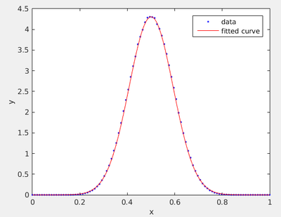
This is impressive, we have an essentially exact result, as far as the eye can see. This was obtained on my machine in 75s. Now we can check the quality of our estimator:
>> std(data)

ans =

    0.0912
vs
f =

     General model:
     f(x) = exp(-(x-x0).^2/(2*sx^2))/(sqrt(2*pi*sx^2))
     Coefficients (with 95% confidence bounds):
       sx =    -0.09268  (-0.09298, -0.09239)
       x0 =      0.5003  (0.4999, 0.5006)
>> std(distribution)
Let us do the same with cases we know do not work (average over 1 or 2 numbers) or for which we are not so sure (average over 3 numbers). This is for 3:
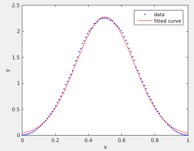
It might not look striking, but this is not a good fit. There is obvious statistical noise (near the top) but there is also unmistakable failure of the fitting function which has the wrong concavity.
The sum of three random numbers is not Normally distributed!
In fact the sum of $N$ random numbers is a piece-wise $N$th order polynomial function, known as the Irwin-Hall distribution.
Here one can have fun fitting with 'gauss8' (the maximum provided) that will typically also fail badly, by taking its added degrees of freedom to fit the noise, while still failing to capture the overall smooth shape of the mysterious function (if you remember the previous lecture you can derive it from the mere convolution of a linear function and a constant one).
Least squares
In the 18th, it was discovered that a good way to approach ideal but unknown models was by minimizing the squares of the residuals between the imperfect observation and the best theory candidate. The residual is merely the difference between what the theory expects and what the observer observes. So if we have $N$ data points $y_1$, ..., $y_N$ obtained for the values $x_1$, ..., $x_N$ that we expect are accounted for by the "model" $f$, i.e., a function $f(x;\beta)$ of $\nu$ parameters $\beta_1$, ..., $\beta_\nu$:
$$r_i=f(x_i;\beta)-y_i\,.$$
We want to minimize the sum of the squared residuals:
$$S=\sum_{i=1}^N r_i^2\,.$$
This we do by varying $\beta$s such that $S$ is minimum, which is achieved when each $\partial S/\partial\beta_j$ term for $1\le j\le\nu$ is canceled independently.
$$\frac{\partial S}{\partial\beta_j}=2\sum_i(f(x_i;\beta)-y_i)\frac{\partial f(x_i;\beta)}{\partial\beta_j}=0\,,\quad\text{for $j=1,\dots,\nu$}\,.\label{eq:lstsq}$$
This is a complicated problem in general, that typically requires iterations over trials and errors.
Linear least square
There is a case where Eq. \ref{eq:lstsq} is considerably simplified, namely, if the partial derivative can be cancelled out, which occurs for so-called linear least squares where the parameters $\beta$ are merely linear coefficients of functions (that can be, of course, nonlinear). That is to say, our test function reads:
$$f(x;\beta)=\sum_{k=1}^\nu\beta_k\phi_k(x)\,,$$
in which case:
$$\frac{\partial f(x_i;\beta)}{\partial\beta_j}=\phi_j(x_i)\,.$$
We put this back in each term of the differential in $\beta$:
$$\sum_{i=1}^N(\sum_{k=1}^\nu\beta_k\phi_k(x_i)-y_i)\phi_j(x_i)=0$$
and now, it remains to rearrange this equality so that we can write it in matrix form. To do so, we have to remember these properties (and notations):
Concatenation:
$$\sum_k A_{ik}B_{kj}=(AB)_{ij}$$
Transposition:
$$A^T_{ij}=A_{ji}$$
so that our equation above becomes:
$$\sum_{i=1}^N\sum_{k=1}^\nu\beta_k\phi_k(x_i)\phi_j(x_i)=\sum_{i=1}^N y_i\phi_j(x_i)\,,$$
We introduce the matrix $\Phi$ such that:
$$\Phi_{ij}=\phi_j(x_i)\label{eq:phi}\,,$$
in which case, with some further grouping and reassembling:
$$\sum_{k=1}^\nu\sum_{i=1}^N\Phi^T_{ji}\Phi_{ik}\beta_k=\sum_{i=1}^N \Phi_{ij}y_i\,,$$
So that we can get rid of the $i$ indices:
$$\sum_{k=1}^\nu(\Phi^T\Phi)_{jk}\beta_k=(\Phi^T y)_j\,,$$
where $y=(y_1,\dots,y_N)^T$, and now getting rid of $k$:
$$[(\Phi^T\Phi)\beta]_j=(\Phi^T y)_j\,,$$
with $\beta$ our vector of unknown parameters. As the equality holds for all $1\le j\le\nu$, it holds for the full vector, providing us with the final equation in its matrix form:
$$(\Phi^T\Phi)\beta=\Phi^T y\,.$$
Assuming $(\Phi^T\Phi)$ is well conditioned (in particular, not singular), we get the formal solution by brute force inversion:
$$\beta=(\Phi^T\Phi)^{-1}\Phi^T y\,.$$
The $(\Phi^T\Phi)^{-1}\Phi^T$ could be problematic if large (many fitting functions and/or many data points) and actually computed in this form, in which case one can see it as the notation for a so-called "pseudo-inverse" that deals with such an object in an efficient and stable way.
Let us now turn from the general theory to a particular example. A convenient basis of function is that of polynomials, that is:
$$f(x;\beta)\equiv\sum_{k=0}^N\beta_k x^k$$
and our $\Phi$ matrix (which by the way goes by the name of a Gramian) reads:
$$\Phi=\pmatrix{ 1 & x_1 & x_1^2 & x_1^3 & \dots \\ 1 & x_2 & x_2^2 & x_2^3& \dots \\ \vdots & & & & \vdots \\ 1 & x_N & x_N^2 & x_N^3 & \dots }$$
Let us try with matlab.
Npts = 10; % number of points
Order = 4; % order of the fit

x=1:Npts;

data=(5*x/Npts).^3+(5*rand(Npts,1))'; % generate noisy data

hold off
plot(data,'o')

%% Fit to order Order
mat = zeros(Npts,Order)
for i=1:Npts
    for j=1:Order
        mat(i,j)=i^(j-1)
    end
end

coeffs=(inv(transpose(mat)*mat)*mat'*data')'
hold on

plot (x,coeffs(1)+coeffs(2)*x+coeffs(3)*x.^2+coeffs(4)*x.^3, 'LineWidth',2)
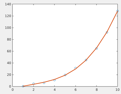
These are our coefficients:
coeffs =

   -3.7674    4.9002   -0.9674    0.1795
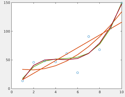
Even if the fit is not very good, it is the optimum one for the choice of functions we made. More functions typically would provide a better fit, although this might not be relevant:
Analytical results
Importantly, whenever we can avoid the computer, we should do so. When fitting with a linear function, of the type:
$$f(x;\beta)=\beta_0+x\beta_1$$
then our matrices become simply:
$$\Phi^T\Phi=\pmatrix{ 1 & 1 & 1 & \dots\\ x_1 & x_2 & x_3 & \dots }\pmatrix{ 1 & x_1 \\ 1 & x_2 \\ 1 & x_3 \\ \vdots & \vdots } = \pmatrix{ N & \sum x_i\\ \sum x_i & \sum x_i^2 }\,,$$
The inverse of a $2\times2$ matrix is the inverse of its determinant times the matrix where diagonal elements are swapped and off-diagonal ones are changed sign, so:
$$(\Phi^T\Phi)^{-1} = \frac{1}{N\sum x_i^2-(\sum x_i)^2} \pmatrix{ \sum x_i^2 & -\sum x_i\\ -\sum x_i & N }\,, $$
and since:
$$\Phi^T y=\pmatrix{ \sum y_i \\ \sum x_iy_i }$$
this brings us to the final, so-called closed-form result:
$$\beta=(\Phi^T\Phi)^{-1}\Phi^T y= \frac{1}{N\sum x_i^2-(\sum x_i)^2} \pmatrix{ \sum x_i^2\sum y_i-\sum x_i\sum x_iy_i \\ -\sum x_i\sum y_i + N\sum x_iy_i& }\,, $$
which is also exact, but remains so even without the computer. These formulas are used by your colleagues in the laboratory sessions. In the chemistry course, we tell them that "this is theory" and do not show them the origin of these results. But you can.
Nonlinear least squares
One can use the linear squares rigorously as long as the coefficients $\beta$ are linear. Sometimes it could appear there is a clever trick to extend its reach of action. Say we have data distributed according to (lifetimes of a radioactive sample of size $N(0)$):
$$N(t)=N(0)\exp(-\gamma t)$$
Then we could do the trick:
$$\ln(N(t))=\ln(N(0))-\gamma t$$
which is a linear function of the coefficients $(\ln N(0), \gamma$) and we could even use the analytical results above.
Tricks can be clever or they can be foolish and deceiving.
In this case, this is considered bad practice (although it could handy for a good-enough job quickly done). However, the noise is not distributed linearly, due to the nonlinear nature of the function. Therefore the regression analysis (the linear least square) will bias the data. Explore this case as an exercise by fitting nonlinearly and using the exact result above. For each time generate a cloud of data so that you can get access to the noise as well, and fit the mean as function of time. (You can also use the exprnd() function to simulate decay times.)
numpts=25000; % number of experiments
dt=1-.05; % probability of no-decay

tdecay=zeros(numpts,1);

for nt=1:numpts
    td=0; % time of decay
    while rand()<dt
        td=td+1;
    end
    tdecay(nt)=td;
end

m=max(tdecay)

nump=25;
partition=linspace(0,m,nump);
dist=histcounts(tdecay,partition);

hold off
%semilogy(dist,'o-')
x=linspace(0,partition(end),nump-1);

plot(x,dist,'o-')

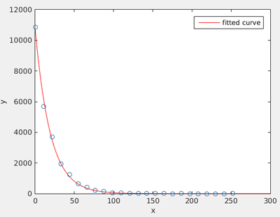
f = fit(x',dist','exp1') %,'StartPoint',[tdecay(1),-1])

hold on
plot(f)
set(gca,'YScale','log')
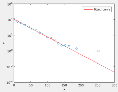
Clearly, seen as a line on the log plot, this is not a good fit! While it is in fact excellent, as seen on the linear-axes figure, because the long time events are rare, and thus have more noise.
Nonlinear Gaussian fit
In the case of Gaussian fit, our model function is (we do not take the norm a fitting parameter as we want to constrain it to 1):
To find the $\mu$ and $\sigma$ that give the best $r_i=f(x_i;\mu,\sigma)-y_i$ that minimizes $S=\sum_{i=1}^N r_i^2$, we look for $dS=0$ and arrive, as before, to $dS=\frac{\partial S}{\partial \mu}d\mu+\frac{\partial S}{\partial \sigma}d\sigma$.
We compute one of these integrals for illustration:
We can start with an initial value for $\mu$ and $\sigma$ and iterate the process until we get close enough. Try this as an exercise. Typically, this will depend crucially on the initial condition.
| Computación I |
|---|
