The two level system: fermionic states

Excitons cannot be described in all regimes by an HO. When density is high enough to push together more than one electron or hole in the same state, the Pauli Exclusion Principle enters the picture. This is also the case of atoms, whose excitations are electronic and therefore saturable. In all these examples, the system can only populate a finite number of levels with a maximum of one excitation. The most suitable description is in terms of the projector operators:^2.7

$\displaystyle \ket{i}\bra{i}$

(2.39)

for each level (with corresponding energy $\omega_i$ ) and their ladder counterparts,

$\displaystyle \ud{\sigma_{ij}}=\ket{j}\bra{i}\,,$

(2.40)

the rising (if $\omega_i<\omega_j$ ) and lowering (if $\omega_i>\omega_j$ ) operators. Eq. (2.40) describes the promotion from state

to $j\neq i$ by creating an excitation of the matter field in the same way as $\ud{a}$ does for the bosonic field. The difference is that $\ud{\sigma_{ij}}$ cannot be applied twice because only one excitation is allowed in each level:^2.8

$\displaystyle \langle i \vert j\rangle=\delta_{ij}\,.$

(2.41)

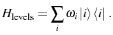
The free Hamiltonian of these levels is simply

$\displaystyle H_\mathrm{levels}=\sum_{i}\omega_{i}\ket{i}\bra{i}\,.$

(2.42)

Let us consider two of these levels with an energy difference of $\omega_\sigma$ and operators of creation and destruction $\ud{\sigma}$ and $\sigma$ respectively. This two-level system (2LS) covers the Fermi statistics in the same way as the HO covers Bose statistics. Together, they describe a great deal of physical situations, as we will see, and, most importantly, they constitute the paradigm for the study of light-matter interaction. For what concerns us, the 2LS is a reasonable approximation for an exciton in a small quantum dot. The two levels involved are the ground state $\ket{0}$ , in the absence of an exciton, and the excited state $\ket{1}=\ud{\sigma}\ket{0}$ , in its presence. The $\sigma$ -operators

$\displaystyle \{\ud{\sigma}=\ket{1}\bra{0},\,\sigma=\ket{0}\bra{1},\,\ud{\sigma}\sigma=\ket{1}\bra{1},\,\sigma\ud{\sigma}=\ket{0}\bra{0}\}$

(2.43)

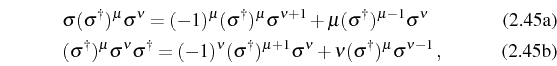
can be put in terms of the pseudo-spin operators or Pauli matrices, $\{s_x,s_y,s_z\}$ :

$\displaystyle \begin{eqnarray}s_z&=&\frac{1}{2}[\ud{\sigma},\sigma]\,,\\ s_x&=&\ud{\sigma}+\sigma\,,\\ s_y&=&-i(\ud{\sigma}-\sigma)\,, \end{eqnarray}$

(2.44a)

used for the

-spin dynamics. The anti-commutation rules^2.9

$\displaystyle [\sigma,\ud{\sigma}]_+=1$

(2.45)

summarizes the fermionic properties of the 2LS algebra. Other useful relations for normal ordering that can be derived from this algebra, are:

$\begin{subequations}\begin{align}&\sigma(\ud{\sigma})^\mu\sigma^\nu =(-1)^\mu(\u... ...}\sigma^\nu+\nu (\ud{\sigma})^\mu\sigma^{\nu-1}\,, \end{align}\end{subequations}$

for $\mu$ , $\nu\in\{0,1 \}$ . From here it is clear that $\sigma\ud{\sigma}\sigma=\sigma$ and $\ud{\sigma}\sigma\ud{\sigma}=\ud{\sigma}$ .

The Hamiltonian in Eq. (2.42) can be written as

$\displaystyle H_\sigma=\omega_\sigma\ud{\sigma}\sigma\,.$

(2.47)

A general state is described by the -dimensional density matrix. It is characterized by two numbers: the probability of having an excitation, which is also the average occupation $\mathcal{P}_1=\langle\ud{\sigma}\sigma\rangle =\langle n_\sigma\rangle$ , and the coherence between the two levels, $\rho^\sigma_{01}$ ,

$\displaystyle \rho^\sigma=\left( \begin{matrix}1-\langle n_\sigma\rangle &\rho^\sigma_{01}\\ (\rho_{01}^\sigma)^*&\langle n_\sigma\rangle \end{matrix}\right)\,.$

(2.48)

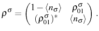
In case of a pure state of the form $\sqrt{1-\langle n_\sigma\rangle }\ket{0}+e^{i\phi_1}\sqrt{\langle n_\sigma\rangle }\ket{1}$ , we have $\rho^\sigma_{01}=\sqrt{\langle n_\sigma\rangle (1-\langle n_\sigma\rangle )}e^{-i\phi}$ . On the other hand, if the system is in thermal equilibrium with some bath at temperature

, we have a thermal mixture as it was the case with bosons. The density matrix of Eq. (2.27) should be computed now taking into account the Fermi-Dirac statistics:

$\displaystyle \rho^\sigma_\mathrm{th}=\frac{e^{-\frac{\omega_\sigma\ud{\sigma}\... ...-\langle n_\sigma\rangle )\ket{0}\bra{0}+\langle n_\sigma\rangle \ket{1}\bra{1}$

(2.49)

where $\langle n_\sigma\rangle$ is the Fermi-Dirac distribution,

$\displaystyle \langle n_\sigma\rangle =\frac{1}{e^{\frac{\omega_\sigma}{k_BT}}+1}\,.$

(2.50)

The maximum value that this probability can take, for infinite temperature, is

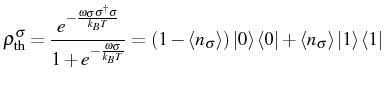
. It is, therefore, not possible to saturate the 2LS, that is, to invert its population, only with a thermal bath. We will see in Sec. 2.4 how this can change when more than one bath is considered.

The thermal equilibrium for the mean value $\langle n_\sigma(t)\rangle$ is driven by the interplay of outgoing particles into the reservoir, with a rate given by $\kappa_\sigma (1+\bar n_T)\langle n_\sigma(t)\rangle$ ( $\kappa_\sigma$ is the Einstein A-coefficient), and incoming particles, at the rate $\kappa_\sigma \bar n_T [1-\langle n_\sigma(t)\rangle ]$ . The incoming rate is, in contrast with the bosonic case, proportional to the subtraction $1-\langle n_\sigma(t)\rangle$ , which is the probability of the system being in the ground state and therefore available for excitation. This provides the saturation effect, as now, with the same definition for the effective parameters as in the previous section, $\gamma_\sigma=\kappa_\sigma (1+ \bar n_T)$ and $P_\sigma=\kappa_\sigma \bar n_T$ (the Einstein B-coefficient), the rate equations reads:

$\displaystyle \frac{d\langle n_\sigma(t)\rangle }{dt}=-\gamma_\sigma\langle n_\sigma(t)\rangle +P_\sigma[1-\langle n_\sigma(t)\rangle ]\,.$

(2.51)

The SS of Eq. (2.50) can be also written as

$\displaystyle n_\sigma^{\mathrm{SS}}=\frac{P_\sigma}{\gamma_\sigma+P_\sigma}=\frac{\bar n_T}{2\bar n_T+1}\,.$

(2.52)

At very high temperatures, as the total income approaches the outcome, $P_\sigma\approx\gamma_\sigma$ , we obtain the half saturation. In this case, the 2LS cannot have the same occupation number as the reservoir, which is bosonic, but both correspond to the same temperature. Also in contrast with the bosonic case, not all possible combinations of the parameters $\gamma_\sigma$ , $P_\sigma$ correspond to a physical thermal bath (where $\gamma_\sigma>P_\sigma$ ). In this text, we will study the most general case of pumping and decay where it is made possible that $P_\sigma>\gamma_\sigma$ , and therefore to completely saturate the 2LS, $n_\sigma^{\mathrm{SS}}=1$ . We will see in Sec. 2.4 how this is feasible experimentally.

It is interesting to note that the 2LS dynamics is symmetric under the exchange of pump and decay ( $\gamma_\sigma\leftrightarrow P_\sigma$ ) if we also exchange the ground and the excited states. Saturation can occur in two senses, in the ground state when the decay is large, and in the excited state when the pump is large. The equivalence between pump and decay for the 2LS is in contrast with the totally different nature that they bear in the HO, where the pump can put up to infinite excitations (when $P_a\rightarrow\gamma_a$ ) but the decay can only ``saturate'' the system in the ground state.