m |
m |
||
| Line 9: | Line 9: | ||
You may need to install packages, which can be done as follows: | You may need to install packages, which can be done as follows: | ||
| − | < | + | <syntaxhighlight lang="python"> |
import Pkg; Pkg.add("Distributions") | import Pkg; Pkg.add("Distributions") | ||
| − | </ | + | </syntaxhighlight> |
Once this is done (once for ever on a given machine), you can then be: | Once this is done (once for ever on a given machine), you can then be: | ||
| − | < | + | <syntaxhighlight lang="python"> |
using Distributions | using Distributions | ||
| − | </ | + | </syntaxhighlight> |
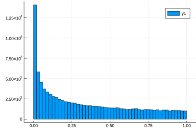
Let us generate ten thousands random points following a squared-uniform probability distribution, $X^2$. | Let us generate ten thousands random points following a squared-uniform probability distribution, $X^2$. | ||
| − | < | + | <syntaxhighlight lang="python"> |
lst=[rand()^2 for i=1:10^5] | lst=[rand()^2 for i=1:10^5] | ||
| − | </ | + | </syntaxhighlight> |
and after | and after | ||
| − | < | + | <syntaxhighlight lang="python"> |
using Plots | using Plots | ||
histogram(lst) | histogram(lst) | ||
| − | </ | + | </syntaxhighlight> |
<center><wz tip="Distribution of $10^5$ squared random numbers.">[[File:julia-randX2.png|400px]]</wz></center> | <center><wz tip="Distribution of $10^5$ squared random numbers.">[[File:julia-randX2.png|400px]]</wz></center> | ||
Revision as of 12:28, 11 February 2020
Crash course in Julia (programming)
Julia is a powerful/efficient/high-level computer programming language. You can get into interacting mode right-away with:
julia
You may need to install packages, which can be done as follows:
import Pkg; Pkg.add("Distributions")
Once this is done (once for ever on a given machine), you can then be:
using Distributions
Let us generate ten thousands random points following a squared-uniform probability distribution, $X^2$.
lst=[rand()^2 for i=1:10^5]
and after
using Plots
histogram(lst)

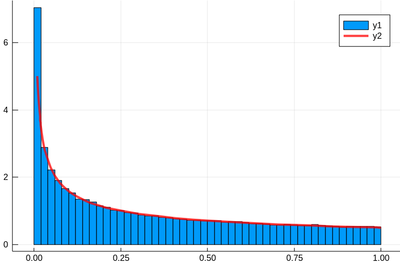
The theoretical result is obtained by differentiating the cumulative function, $f_{X^2}=dF_{X^2}/dx$, with
$$F_{X^2}(x)\equiv\mathbb{P}(X^2\le x)$$
but $\mathbb{P}(X^2\le x)=\mathbb{P}(X\le\sqrt{x})=\sqrt{x}$, since the probability is uniform. Therefore:
$$f_{X^2}(x)={1\over2\sqrt{x}}$$
Let us check:
f(x)=1/(2*sqrt(x))
histogram(lst,norm=true)
plot!(f,.01,1, linewidth = 4, linecolor = :red, linealpha=0.75)
The ! means to plot on the existing display. This seems to work indeed:
