m |
m |
||
| Line 54: | Line 54: | ||
<center><wz tip="Comparison of the normalized histogram with the theoretical result.">[[File:julia-randX2th.png|400px]]</wz></center> | <center><wz tip="Comparison of the normalized histogram with the theoretical result.">[[File:julia-randX2th.png|400px]]</wz></center> | ||
| − | Let's have a look at the distribution of inverse random numbers, also sampled from a uniform distribution between 0 and 1. This time, the support is infinite (it is $[1,\infty[$). | + | Let's have a look at the distribution of inverse random numbers, also sampled from a uniform distribution between 0 and 1. This time, the support is infinite (it is $[1,\infty[$). The theoretical distribution is $f_{1/X}=d\mathbb{P}_{1/X}/dx$ with |
| + | $\mathbb{P}_{1/X}=\mathbb{P}(1/X\le x)=\mathbb{P}(X\ge 1/x)=1-1/x$ (being uniform again), so that $f_{1/X}(x)=1/x^2$. | ||
| + | |||
| + | This time we'll use a lot of points to make sure we get the exact result: | ||
| + | |||
| + | <syntaxhighlight lang="python"> | ||
| + | @time lst = [1/rand() for i=1:10^8] | ||
| + | </syntaxhighlight> | ||
| + | |||
| + | The @time allows us to benchmark the time and memory resources involved. As you can see, on a [[2020]] [[caliz|machine]], it's pretty fast (for a hundred million points!) | ||
| + | |||
| + | <pre> | ||
| + | 0.427357 seconds (67.69 k allocations: 766.257 MiB, 0.65% gc time) | ||
| + | </pre> | ||
| + | |||
| + | The result is also consequently very smooth: | ||
| + | |||
| + | <syntaxhighlight lang="python"> | ||
| + | @time histogram(lst,norm=true,bins=0:.01:10) | ||
| + | </syntaxhighlight> | ||
| + | |||
| + | returning | ||
| + | |||
| + | <pre> | ||
| + | 4.644046 seconds (4.88 k allocations: 1.490 GiB, 1.74% gc time) | ||
| + | </pre> | ||
| + | |||
| + | and, after also | ||
| + | |||
| + | <syntaxhighlight lang="python"> | ||
| + | f(x)=1/x^2 | ||
| + | plot!(f,1,10,linewidth=4,linecolor=:red,linealpha=.75) | ||
| + | </syntaxhighlight> | ||
| + | |||
| + | <center><wz tip="Distribution of 100 million inverses of random points and its slightly off theoretical fit.">[[File:Screenshot_20200211_125427.png|400px]]</wz></center> | ||
| + | |||
| + | This is slightly off, clearly. The culprit is our distribution function, which density should be 1 at x=1 and is more than that. The problem is the norm option of histogram, that normalizes to what is plotted (or retained). And we have points beyond that. We can use this number to renormalize our theory plot. This is how many numbers we have: | ||
| + | |||
| + | <syntaxhighlight lang="python"> | ||
| + | sum(lst .< 10) | ||
| + | </syntaxhighlight> | ||
| + | |||
| + | and this is the list of these numbers: | ||
| + | |||
| + | <syntaxhighlight lang="python"> | ||
| + | lst[lst .> 100] | ||
| + | </syntaxhighlight> | ||
| + | |||
| + | Let us now explore numerically a very interesting (and important) phenomenon. For that, we'll need the Cauchy function from the above-loaded "Distributions" package. This is a histogram of $10^5$ Cauchy-distributed points: | ||
| + | |||
| + | <syntaxhighlight lang="python"> | ||
| + | histogram(rand(Cauchy(),10^5)) | ||
| + | </syntaxhighlight> | ||
| + | |||
| + | <center><wz tip="Distribution of $10^5$ Cauchy-distributed points. Not good.">[[File:Screenshot_20200211_141839.png|400px]]</wz></center> | ||
| + | |||
| + | Here the binning is mandatory: | ||
| + | |||
| + | <syntaxhighlight lang="python"> | ||
| + | histogram(rand(Cauchy(),10^5),bins=-10:.5:10,norm=true) | ||
| + | </syntaxhighlight> | ||
| + | |||
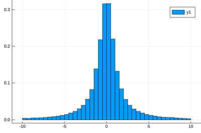
| + | <center><wz tip="Same as above, within boundaries!">[[File:Screenshot_20200211_142148.png|400px]]</wz></center> | ||
Revision as of 14:24, 11 February 2020
Crash course in Julia (programming)
Julia is a powerful/efficient/high-level computer programming language. You can get into interacting mode right-away with:
julia
You may need to install packages, which can be done as follows:
import Pkg; Pkg.add("Distributions")
Once this is done (once for ever on a given machine), you can then be:
using Distributions
Let us generate ten thousands random points following a squared-uniform probability distribution, $X^2$.
lst=[rand()^2 for i=1:10^5]
and after
using Plots
histogram(lst)
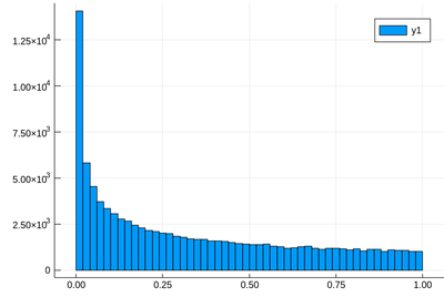
The theoretical result is obtained by differentiating the cumulative function, $f_{X^2}=dF_{X^2}/dx$, with
$$F_{X^2}(x)\equiv\mathbb{P}(X^2\le x)$$
but $\mathbb{P}(X^2\le x)=\mathbb{P}(X\le\sqrt{x})=\sqrt{x}$, since the probability is uniform. Therefore:
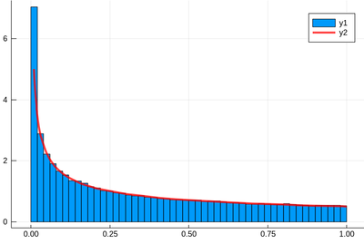
$$f_{X^2}(x)={1\over2\sqrt{x}}$$
Let us check:
f(x)=1/(2*sqrt(x))
histogram(lst,norm=true)
plot!(f,.01,1, linewidth = 4, linecolor = :red, linealpha=0.75)
The ! means to plot on the existing display. This seems to work indeed:
Let's have a look at the distribution of inverse random numbers, also sampled from a uniform distribution between 0 and 1. This time, the support is infinite (it is $[1,\infty[$). The theoretical distribution is $f_{1/X}=d\mathbb{P}_{1/X}/dx$ with $\mathbb{P}_{1/X}=\mathbb{P}(1/X\le x)=\mathbb{P}(X\ge 1/x)=1-1/x$ (being uniform again), so that $f_{1/X}(x)=1/x^2$.
This time we'll use a lot of points to make sure we get the exact result:
@time lst = [1/rand() for i=1:10^8]
The @time allows us to benchmark the time and memory resources involved. As you can see, on a 2020 machine, it's pretty fast (for a hundred million points!)
0.427357 seconds (67.69 k allocations: 766.257 MiB, 0.65% gc time)
The result is also consequently very smooth:
@time histogram(lst,norm=true,bins=0:.01:10)
returning
4.644046 seconds (4.88 k allocations: 1.490 GiB, 1.74% gc time)
and, after also
f(x)=1/x^2
plot!(f,1,10,linewidth=4,linecolor=:red,linealpha=.75)
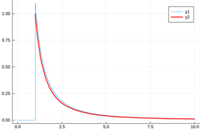
This is slightly off, clearly. The culprit is our distribution function, which density should be 1 at x=1 and is more than that. The problem is the norm option of histogram, that normalizes to what is plotted (or retained). And we have points beyond that. We can use this number to renormalize our theory plot. This is how many numbers we have:
sum(lst .< 10)
and this is the list of these numbers:
lst[lst .> 100]
Let us now explore numerically a very interesting (and important) phenomenon. For that, we'll need the Cauchy function from the above-loaded "Distributions" package. This is a histogram of $10^5$ Cauchy-distributed points:
histogram(rand(Cauchy(),10^5))
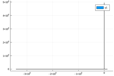
Here the binning is mandatory:
histogram(rand(Cauchy(),10^5),bins=-10:.5:10,norm=true)
