Spontaneous Emission

In the most general case of SE, the $D^\mathrm{SE}$ coefficient at resonance, $D_0^\mathrm{SE}$ , is a complex number. If the initial condition further fulfils $\Re n_{ab}^0=0$ , it becomes pure imaginary. Usually [see the work by Carmichael et al. (1989), Andreani et al. (1999)], the initial states considered are independent states of photons or excitons (not a quantum superposition), where indeed $n_{ab}^0=0$ . In these cases,

$\displaystyle D_0^\mathrm{SE}=i\frac{\frac{g}{2}(\gamma_an^0_b-\gamma_bn^0_a)}{g^2(n_a^0+n_b^0)+n_a^0\gamma_b\gamma_+}\,,$

(3.55)

which yields the following expression for the spectrum:

$\displaystyle S_0^\mathrm{SE}(\omega)=\frac{1}{\pi} \frac{\frac{\gamma_a + \gam... ...(g^2 (n_a^0 + n_b^0) + n_a^0 \gamma_b \frac{\gamma_a + \gamma_b}{4} \right)}\,.$

(3.56)

The SE spectrum of exciton observed in the leaky modes is obtained from Eq. (3.59) by exchanging the indexes $a\leftrightarrow b$ . We illustrate this with the two particular cases that follow.

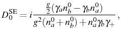
The typical detection geometry for the spontaneous emission of an atom in a cavity consists in having the atom in its excited state as the initial condition, and observing its direct emission spectrum. In this case the role of the cavity is merely to affect the dynamics of its relaxation, that is oscillatory with the light-field in the case of SC. This case corresponds to $n^0_{b}=1$ and $n^0_{a}=n^0_{ab}=0$ in Eq. (3.59) with $a\leftrightarrow b$ . This gives:

$\displaystyle S_0^\mathrm{SE}(\omega)=\frac{1}{\pi} \frac{\frac{\gamma_a + \gam... ...amma_{a} \frac{\gamma_a + \gamma_b}{4})(g^2 + \frac{\gamma_a\gamma_b}{4})^2}\,.$

(3.57)

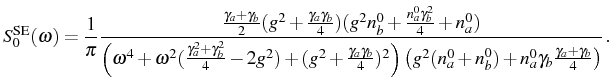
In the semiconductor case, one would typically still have in mind the excited state of the exciton as the initial condition, but this time, this is the cavity emission that is probed. The initial condition is therefore the same as before but without interchanging and in Eq. (3.59), which reads in this case:

$\displaystyle S_0^\mathrm{SE}(\omega)=\frac{1}{\pi}\frac{2(\gamma_a+\gamma_b)(4... ...{16\omega^4-4\omega^2(8g^2-\gamma_a^2-\gamma_b^2)+(4g^2+\gamma_a\gamma_b)^2}\,.$

(3.58)

The difference in the lineshape due to the initial quantum state is seen in Fig. 3.6. The visibility of the line-splitting is much reduced in the case of an exciton in SC which SE is detected through the cavity emission, than in the case of a photon, due to a larger dispersive contribution to the spectrum in the second case. The reason for such a strong interference term is that the photon is the most dissipative mode in this example (where $\gamma_a>\gamma_b$ ) and, therefore, when the system is ``more photonic'' (initiated as a photon) the overlap between polaritons is more pronounced. With a polariton as an initial state, only one line is produced.

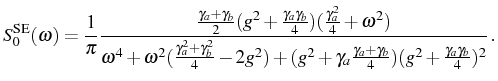
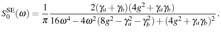
Again, by symmetry, interchanging $a\leftrightarrow b$ in Eqs. (3.60) and (3.61), correspond to the SE of the system prepared as a photon at the initial time and detected in, respectively, the cavity emission on the one hand (Eq. (3.60), $a\leftrightarrow b$ ), and in the leaky mode emission on the other hand [Eq. (3.61)]. In the latter case, the spectrum is invariant under the exchange $a\leftrightarrow b$ . Fig. 3.6 also hints to the changes brought by the detection channel (direct emission of the exciton or through the cavity mode).

If or (in which case $n^0_{ab}=0$ ), the normalized spectra do not depend on the nonzero value or . That is, one cannot distinguish in the lineshape, the decay of one exciton from that of two, or more. In the more general case, when $n_{ab}^0\neq0$ , the peaks can be differently weighted. For instance, starting with an upper polariton $\vert\mathrm{U}\rangle=(\vert 1,0\rangle+\vert,1\rangle)/\sqrt{2}$ ( $n_{a}^0=n_b^0=n_{ab}^0=1/2$ ) gives rise to a dominant upper-polariton peak (labelled 2 in the above equations, as seen in the brown dotted line in Fig. 3.6). One can classify the possible lineshapes obtained for various initial states. For instance, as we have just mentioned, the normalized spectrum of $\ket{0,n}$ as an initial state, is the same whatever the nonzero , which is not unexpected from a linear model. From the previous statement, the same spectrum is also obtained for a coherent state or a thermal state of photons, or indeed any quantum state, as long as the exciton population remains zero. In the same way, the PL spectrum of the product of coherent states in the photon and exciton fields, $\ket{z}\ket{z'}$ with $z=z'\in\mathbb{C}^*$ , is the same as that of a polariton state $\vert\mathrm{U}\rangle$ , although both are very different in character: a classical state on the one hand and a maximally entangled quantum state on the other.