Effective Hamiltonian close to the two-photon resonance

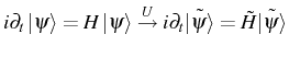
In order to derive an effective Hamiltonian, first, we make a change of the reference frame to the cavity frequency $\omega_a$ . The unitary operator of the transformation reads $U=\exp(-i\omega_a(\ud{a}a+\sum_j \ud{\sigma_j}\sigma_j) t)$ , and it is constructed such that

$\displaystyle i\partial_t\ket{\psi}=H\ket{\psi}\stackrel{U}{\rightarrow} i\partial_t\tilde{\ket{\psi}}=\tilde{H} \tilde{\ket{\psi}}$

(6.23)

with $\tilde{\ket{\psi}}=U\ket{\psi}$ and

$\displaystyle \tilde{H}= U H \ud{U}-i U\partial_t\ud{U}= H_0+H_\mathrm{int}$

(6.24)

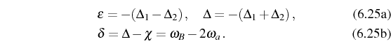
where

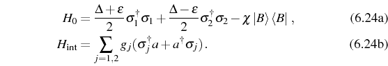
$\begin{subequations}\begin{align}H_0&=\frac{\Delta+\epsilon}{2}\ud{\sigma_1}\sig... ...\sum_{j=1,2} g_j(\ud{\sigma_j}a+\ud{a}\sigma_j)\,. \end{align}\end{subequations}$

Here, we have introduced the detunings

$\begin{subequations}\begin{align}&\epsilon=-(\Delta_1-\Delta_2)\,,\quad \Delta=-... ..._2)\,,\\ &\delta=\Delta-\chi=\omega_B-2\omega_a\,. \end{align}\end{subequations}$

In order to study the new 2PR condition and the strength of the effective coupling that it induces, we take the limit $\vert\Delta\vert\gg g_j,\vert\delta\vert,\vert\epsilon\vert$ , where the 2PR can be achieved and 1PR suppressed. An effective Hamiltonian can be obtained, $H_\mathrm{eff}=H_{\mathrm{eff},2P}+H_{\mathrm{eff},0P}$ , within perturbation theory up to second order, which decouples the subspaces $\mathcal{H}_\mathrm{2P}=\{\ket{G,n},\ket{B,n-2}\}$ (with two photon exchange between states) and $\mathcal{H}_\mathrm{0P}=\{\ket{E1,n},\ket{E2,n}\}$ (with no photon exchange). The effective Hamiltonian for the two photon exchange at fixed excitation number is given by

$\displaystyle H_\mathrm{eff,2P}^{n}=\lambda_{Gn}S_n\ud{S_n}+\lambda_{Bn-2}\ud{S_n}S_n+g_\mathrm{eff}\sqrt{n(n-1)}(\ud{S_n}+S_n)$

(6.27)

with $S_n=\ket{G,n}\bra{B,n-2}$ and the renormalized eigenenergies/coupling constant

$\begin{subequations}\begin{align}&\lambda_{Gn}=-2 n \frac{g_1^2+g_2^2}{\Delta}\,... ...a}\,,\\ &g_\mathrm{eff}=-4\frac{g_1g_2}{\Delta}\,. \end{align}\end{subequations}$

The two photon resonant condition $\lambda_{Gn}=\lambda_{Bn-2}$ , or in terms of detunings,

$\displaystyle \delta_\mathrm{2PR}=-2\frac{g_1^2+g_2^2}{\Delta}\,,$

(6.29)

is independent of the manifold, that is, of the number of photons in the cavity. When this condition is satisfied (for the cavity mode placed at $\omega_a^\mathrm{2PR}=(\omega_B-\delta_\mathrm{2PR})/2$ ), the Hamiltonian is that of an effective 2P exchange through the operator $S=\ket{G}\bra{B}$ :

$\displaystyle H_\mathrm{eff,2P}=\delta_\mathrm{2PR} \ud{a} a+2\delta_\mathrm{2PR} \ud{S}S+g_\mathrm{eff}(\ud{a}^2 S+\ud{S} a^2)\,.$

(6.30)

Similarly, one can determine the effective Hamiltonian in the subspace $\mathcal{H}_\mathrm{0P}$ . In this subspace there is no exchange of energy between QD and cavity and no photon is involved in their Rabi oscillations. The only oscillations taking place in this system when Eq. (6.29) is satisfied and detuning $\Delta$ is infinite, are those of two photons. Moreover, as the two subspaces $\mathcal{H}_\mathrm{0P}$ and $\mathcal{H}_\mathrm{2P}$ are effectively decoupled in this limit, if the system is initiated in a biexcitonic or ground state, only $\mathcal{H}_\mathrm{2P}$ will be populated dominating the dynamics.

**Figure 6.16:** Populations of the QD levels as a function of time with initial state $\ket{G,2}$ : $\ket{B,0}$ (solid-blue line), $\ket{E,1}$ (dashed-purple) and $\ket{G,2}$ (dotted-brown). The parameters for each case are: (a) $\Delta=0$ , $\chi=0$ , (b) $\Delta=5g$ , $\chi=\Delta-\delta_\mathrm{2PR}$ , (c) $\Delta=20g$ , $\chi=\Delta-\delta_\mathrm{2PR}$ , (d) $\Delta=20g$ , $\chi=\Delta$ .
$\includegraphics[width=0.48\linewidth]{chap6/2P/Rabi1/Rabi-d_0-B_0.eps}$ $\includegraphics[width=0.48\linewidth]{chap6/2P/Rabi1/Rabi-d_2.5-B_2.5.eps}$ $\includegraphics[width=0.48\linewidth]{chap6/2P/Rabi1/Rabi-d_10-B_10.eps}$ $\includegraphics[width=0.48\linewidth]{chap6/2P/Rabi1/Rabi-d_10-B_10-no-SS.eps}$

However, for intermediate values of $\vert\Delta\vert$ , in general all the QD levels get populated and 1P oscillations between the subspaces $\mathcal{H}_\mathrm{2P}$ and $\mathcal{H}_\mathrm{0P}$ also take place. Keeping in mind the effective physics that we have just obtained, let us analyze the possible situations depending on the exciton detuning $\Delta$ and the biexciton binding energy $\chi$ , by plotting the Rabi oscillations of the total Hamiltonian. We consider the dynamics inside the manifold with two excitations given by the states $\{\ket{G,2},\ket{E1,1},\ket{E2,1},\ket{B,0}\}$ . The population of each of these states, $\ket{j}$ , from the initial state $\ket{G,2}$ , is given by $\rho_j(t)=\vert\bra{j}e^{-iHt}\ket{G,2}\vert^2$ . We suppose that the coupling constants and detunings of the two excitons are equal (, $\Delta_1=\Delta_2=-\Delta/2$ and $\epsilon=0$ ). In Fig. 6.16, the population of $\ket{B,0}$ is plotted in solid-blue lines, that of $\ket{G,2}$ in dotted-brown, and the sum of the populations of $\ket{E1,1}$ and $\ket{E1,2}$ in dashed-purple. The last magnitude ( $\rho_{E,1}$ ) is the total population in the subspace $\mathcal{H}_\mathrm{0P}$ and it can only interact through 1P exchange with the other subspace. Therefore, its oscillations are all the 1P oscillations occurring in the system. On the other hand, oscillations in populations $\rho_{G,2}$ or $\rho_{B,0}$ are a mixture of 1P and 2P exchanges, only those clearly between $\rho_{G,2}$ and $\rho_{B,0}$ are purely 2P like.

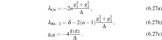
The first case in Fig. 6.16-(a) is that of complete resonance between all QD states and the cavity ( $\Delta=0$ and $\chi=0$ ). All states 1P-oscillate and there are no 2P oscillations due to the destructive interference. When the binding energy of the biexciton is introduced and the 2P resonance condition achieved, 2P oscillations appear already at small detuning, $\Delta=5g$ , in Fig. 6.16-(b). The coupling strength in the second manifold for identical excitons is renormalized twice by a factor $\sqrt{2}$ (i.e., by 2), having as a result a period for the 1P oscillations of $T_{1P}\approx \pi/(2g)$ . 2P oscillations are slower as the Rabi frequency is given by $g_\mathrm{eff}$ and therefore $T_\mathrm{2P}\approx \vert\Delta\vert/2 T_{1P}$ . In this case, it is clear also in the plot that for each 2P oscillations between $\rho_{B,0}$ and $\rho_{G,2}$ , three 1P oscillations take place in $\rho_{E,1}$ . The amplitude of the oscillations is inversely related to the detuning between the cavity mode and the transition involved. 2P oscillations occur almost with maximum amplitude while 1P ones (off-resonance by $\Delta/2$ ) never do. These features are enhanced if the excitonic detuning is increased (keeping the 2P resonance condition) as we can see in Fig. 6.16-(c) where $\Delta=20g$ . Note that the amplitude of the oscillations is practically because we obtain the 2P resonance condition computing and taking into account the Stark shift of the cavity mode due to the presence of the nonresonant excitons. If this shift is not included in the derivation, a naive 2P condition would be simply $\Delta=\chi$ . This would still lead to enhanced 2P oscillations but with a reduced amplitude, as can be seen in Fig. 6.16-(d).

We can conclude from the previous discussion that the larger $\Delta$ , the stronger the 2P oscillations and the more suppressed the 1P oscillations. At a large enough value of $\Delta$ , the result would be the same as using the effective Hamiltonian (where $\rho_{E}\rightarrow0$ for this initial condition). The problem associated with increasing $\Delta$ , as discussed in more details in the following sections, is that the effective coupling also becomes weaker and the cavity must be extremely good to observe such a slow dynamics.

**Figure 6.17:** QD levels as compared to the cavity mode with a biexcitonic energy of $\chi=20g$ . When the cavity mode changes its energy, the situation changes from (a) to (c). In case (a) with $\Delta=0$ ( $\omega_a=\omega_E=\omega_{B}-\omega_E+\chi$ ), there a 1P resonance between $\ket{G}$ and $\ket{E}$ only and no 2PR ( $2\omega_a=\omega_B+\chi$ ). In case (b) with $\Delta=20g$ , there is no 1PR ( $\omega_a=\omega_E-10g=-(\omega_B-\omega_E)-10g$ ) but the system is close to 2PR ( $2\omega_a=\omega_B$ ). In case (c) with $\Delta=2\chi$ ( $\omega_a=\omega_B-\omega_E=\omega_E-\chi$ ), there a 1P resonance between $\ket{E}$ and $\ket{B}$ only and again no 2PR ( $2\omega_a=\omega_B-\chi$ ). In this simple schema the Stark shift is not considered explicitly nor plotted.
$\includegraphics[width=.8\linewidth]{chap6/2P/Levels/levels-cavity-det-letters.eps}$

Getting closer to the experimental situation, we fix the QD energy levels $\omega_1=\omega_2=\omega_E$ and choose a reasonable value for the biexciton energy $\chi=20g$ . We will not speak explicitly the Stark shift in what follows in order to simplify the discussion (writing approximate expressions for the resonance conditions) but it is included for a completely efficient 2PR resonance.

The transition between 1PR and 2PR can be evidenced by tuning the cavity from $\omega_a\approx \omega_E$ to $2\omega_a\approx\omega_B$ . The QD levels corresponding to both cases are plotted in Fig. 6.17-(a) and (b) respectively. The evolution of populations in the manifold with two excitations is again shown in Fig. 6.18 in order to appreciate the qualitative change in the dynamics when tuning the cavity mode. In Fig. 6.18(a), we can see the oscillations in the configuration of Fig. 6.17(a) that correspond to 1P exchange only between states $\ket{G,2}$ and $\ket{E,1}$ . The oscillations in the other extreme configuration of Fig. 6.17(b) are plotted in Fig. 6.16-(d). The intermediate cases where the QD transitions are not in resonance with the energy of 1 nor 2 photons, are those in Fig. 6.18-(b) and (c). We can see that 2P oscillations appear clearly only when the cavity is brought very close to the 2PR condition ( $\Delta \approx \chi$ ). This can be also seen in a more precise way in Fig. 6.19-(a), where we plot the amplitude of the oscillations in the populations as a function of detuning $\Delta$ . The broad peak sitting at $\Delta=0$ affects only populations $\rho_G$ and $\rho_E$ , while at $\Delta \approx \chi$ the peak is very narrow and affects populations $\rho_G$ and $\rho_B$ . The first one corresponds to a 1PR and the second to the 2PR.

**Figure 6.18:** Populations of the QD levels as a function of time with initial state $\ket{G,2}$ : $\ket{B,0}$ (solid-blue line), $\ket{E,1}$ (dashed-purple) and $\ket{G,2}$ (dotted-brown). In all cases the QD levels and biexciton energy are fixed with $\chi=20g$ while the cavity mode changes from 1PR in (a) $\Delta=0$ towards 2PR: (b) $\Delta=10g$ (c) $\Delta=18g$ , (d) $\Delta=19g$ . The perfect 2PR, corresponding to case (b) in Fig. 6.17, can be seen in Fig. 6.16-(c).
$\includegraphics[width=0.45\linewidth]{chap6/2P/Rabi2/Rabi-d_0-B_10.eps}$ $\includegraphics[width=0.45\linewidth]{chap6/2P/Rabi2/Rabi-d_5-B_10.eps}$ $\includegraphics[width=0.45\linewidth]{chap6/2P/Rabi2/Rabi-d_9-B_10.eps}$ $\includegraphics[width=0.45\linewidth]{chap6/2P/Rabi2/Rabi-d_9.5-B_10.eps}$

Note that if the cavity energy is further tuned down to $\Delta\approx 2\chi$ (see Fig. 6.17-(c)), the 1P resonance is again satisfied for the transition between states $\ket{E}$ and $\ket{B}$ . In order to see these oscillations at the Hamiltonian level, the system must be initiated in a state other than $\ket{G,2}$ . That is, a higher excitation intensity is needed to see this second 1PR. In Fig. 6.19-(b), the amplitude of oscillations for the initial state $\ket{B,0}$ , shows a third broad peak at $\Delta\approx 2\chi$ affecting only populations $\rho_E$ and $\rho_B$ . This is the second 1PR. The 2PR also manifests in this configuration in the same way as starting with $\ket{G,2}$ . Finally, if the initial state is a superposition of both cases ( $(\ket{G,2}+\ket{B,0})/\sqrt{2}$ ), the dynamics resulting is a superposition of the previous two cases, where we can see the three resonances with less sharp transitions among them.

**Figure 6.19:** Visibility of the population oscillations of the states of the manifold with two excitations when tuning the cavity energy (changing detuning $\Delta$ ): $\ket{B,0}$ (solid-blue line), $\ket{E,1}$ (dashed-purple) and $\ket{G,2}$ (dotted-brown). Biexciton energy is fixed to $\chi=20g$ . Plot (a) corresponds to oscillations from an initial state $\ket{G,2}$ , (b) from $\ket{B,0}$ , (c) from $(\ket{G,2}+\ket{B,0})/\sqrt{2}$ and (d) from a mixture with $40\%$ of $\ket{B,0}$ and $20\%$ of each of the other states. These curves present some mathematical (not fundamental) noise. Depending on the case, the peaks corresponding to 1PR can be seen at $\Delta\approx0$ (oscillations between $\ket{G}$ and $\ket{E}$ ) or at $\Delta\approx 2\chi$ (between $\ket{E}$ and $\ket{G}$ ). The peak of 2PR manifests in all cases at $\Delta \approx \chi$ .
$\includegraphics[width=0.48\linewidth]{chap6/2P/Amplitudes/Ground-detuning.eps}$ $\includegraphics[width=0.48\linewidth]{chap6/2P/Amplitudes/Biexciton-detuning.eps}$ $\includegraphics[width=0.48\linewidth]{chap6/2P/Amplitudes/BG-detuning.eps}$ $\includegraphics[width=0.48\linewidth]{chap6/2P/Amplitudes/BGMix-detuning.eps}$